Picongpu: longitudinal mesh

[cbontoiu]

Hello,
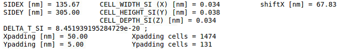
I have a 2D simulation using adios and my mesh sizes should be in the order of 0.03 nm, that is three times smaller than the width of the layers which I want to study.

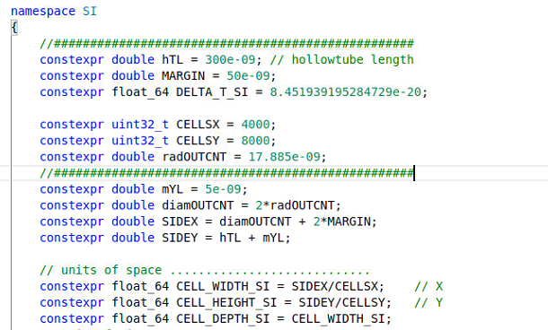
my grid.param file contains

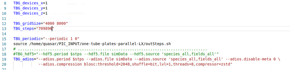
my cfg file contains

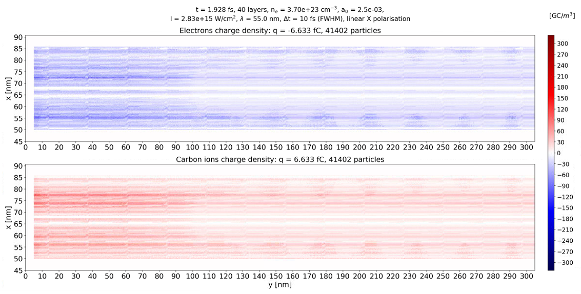
but the charge density plot looks like the longitudinal (y) mesh was about 20 nm large.

Where could the problem be?

[sbastrakov]

Hello @cbontoiu . Your grid.param looks fine for me.

Sorry, I did not understand the question. On the pictures attached, it looks your simulation area size is about 300 nm in Y, as you requested. So where does the 20nm in your question come from? Is it that the ratio of your structure size in Y to grid size is far from what your expected? From the provided information I can only see the grid size and area size

[cbontoiu]

Hello @sbastrakov and thank you for your reply. If you click on the cherge density figure and look along the layers, you will notice that there are some segments about 20 nm long. This make me thing about the accuracy of the data. I mean that data might come truncated at some number of significant digits. Othrwise the charge density along the layers should vary smoothly.

[sbastrakov]

Thanks for explaining. Yes, I see the weird pattern. Do not have an idea where it comes from. Truncation does not occur to me as a likely explanation, though. Can I see your full set of .param files?

[cbontoiu]

Here you have the full folder. Thank you!

one-tube-plates-parallel-LX.zip

[sbastrakov]

I don't see anything suspicious. Compression may be a suspect, I do not have experience with it to evaluate if it's reasonable to suspect this effect from it.

Edit: however it seems to be lossless, then my suggestion is not correct.

[cbontoiu]

I must say that this problem dissapears at later times as you can see in the image below. Interestingly, I can see the effects of ionization by collision, or at least this is what seems to be the cause of the traces arount y = 210 nm. Even more interesting is the appearance of an additional channel of charge depletion on each side of the tube, but this is to be investigated; no error there. It must be something physical and unexplored yet, so PIConGPU is really interesting in what it can show.

[PrometheusPi]

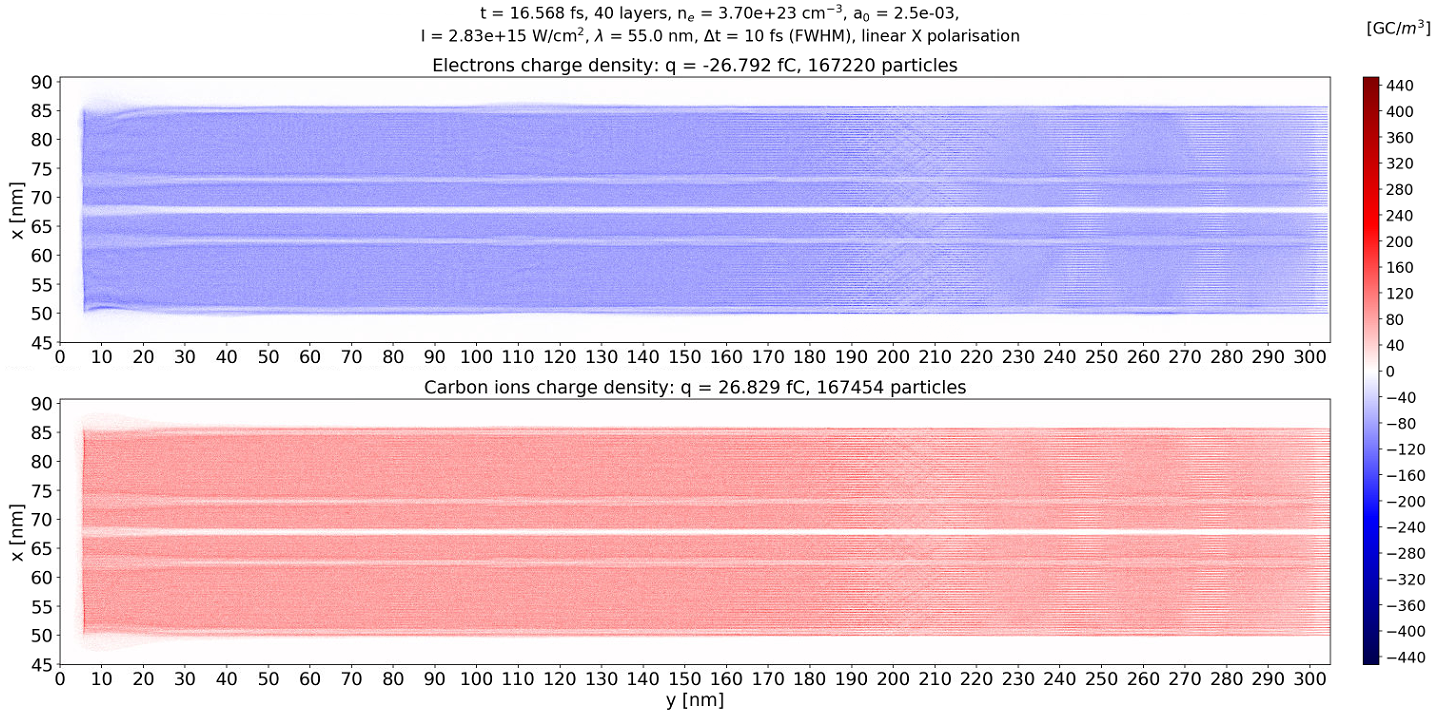
@cbontoiu Do theses structures you observed in your first plot continue to exist if you zoom in? Matplotlib can show some strange artifacts if it rescales fine structures (your data at 4000x8000 pixels) down to screen resolution (something below 1000x1000 pixels).

[cbontoiu]

@PrometheusPi Thank you for your suggestion

I checked at t = 0 when charge density should be all uniform.

The structures are there, even when zoomed.

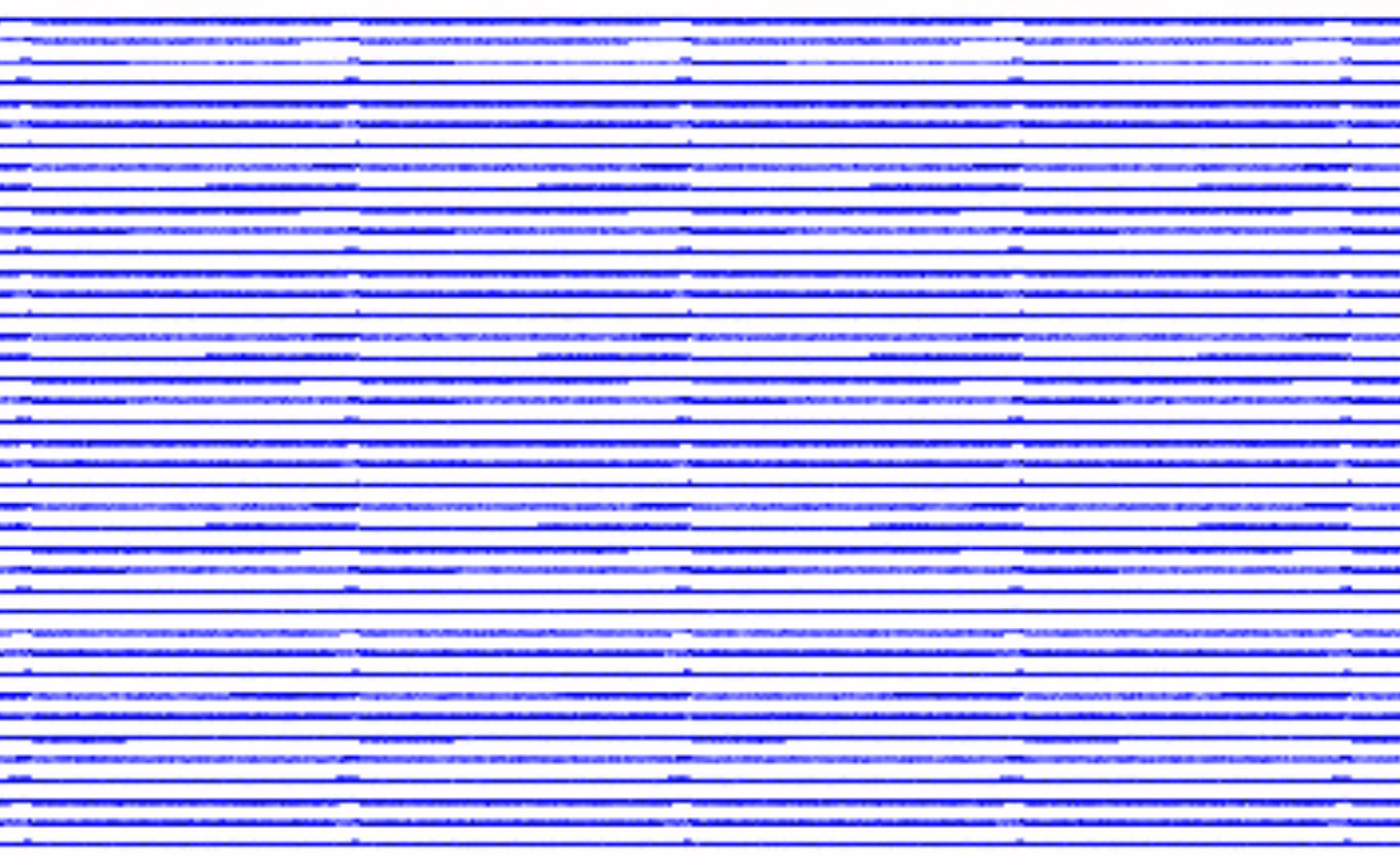
but their axial length is about 10 nm so different than in the first figure of this issue. This makes me think that you are right and it is only something about rendering. I don't plot directly in Jupyter/Matplotlib but instead I write the images on the disk with 150 dpi resolution.

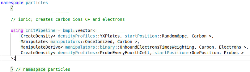
It's fine, I am happy with the longitudinal artifacts but in the zoomed images you can see that there are charge density variations also in in the radial direction within each layer. My explanation so far was that since it must be something related to how the mesh cells interesect the layers. I can see however what seems to be the granularity coming form the number of macroparticles per cell (6 in my case) because in speciesInitialization.param I use CreateDensity< densityProfiles::YXPlates, startPosition::Random6ppc, Carbon >, with the definition in particle.param

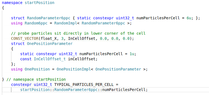
namespace startPosition
{   
    struct RandomParameter6ppc { static constexpr uint32_t numParticlesPerCell = 6u; };
    using Random6ppc = RandomImpl< RandomParameter6ppc >;
    // probe particles sit directly in lower corner of the cell
    CONST_VECTOR(float_X, 3, InCellOffset, 0.0, 0.0, 0.0);
    struct OnePositionParameter  { static constexpr uint32_t numParticlesPerCell = 1u; const InCellOffset_t inCellOffset; };
    using OnePosition = OnePositionImpl< OnePositionParameter >;
} // namespace startPosition
    constexpr uint32_t TYPICAL_PARTICLES_PER_CELL = startPosition::RandomParameter6ppc::numParticlesPerCell;

My guess is that I could do more in order to have the charge distribution across and along the layers more uniform but I don't know how. Maybe working with 12 ppc instead of 6 ppc? I know that this will affect the memory but should increase the resolution during the whole simulation. What would you suggest? What would be the indicator that the number of ppc is acceptable, apart from comparing different results?

[PrometheusPi]

@cbontoiu From the limited knowledge where the artifacts come from, it is hard to suggest something.

In general I would only use more macro particles if the numeric stability requires it - or in other words: to reduce numeric noise caused by the (low) particle sampling. Since you already use 6ppc, the simulation might have encountered a different issue. In PIConGPU we have a minimal weighting. In your case you might have run into the minimum weighting, if you stayed with the default value.
According to your plots, you have ~300GC/m^3. Thus ~300GC/m^-3 / 1.6e-19 C ~2e30 electrons/m^3. If I multiply this with your cell volume:

300e9/1,6e-19 * 0,034e-9 * 0,038e-9 * 0,034e-9 ~0.08

I get a number of 0.08 electrons per cell. Thus, if your minimal weighting is not w_min << 0.08, PIConGPU will reduce the number of macro particles per cell from 6 to 5 and so on until the macro particles fulfill the minimal weighting. In case the minimum weighting is not fulfilled by a single macro-particle, no macro-particle is created and thus your density in the simulation is not sampled, or in other words is assumed to be zero. Increasing the ppc from 6ppc to 12ppc would not solve this problem.

Could you give us your current minimum weighting and the weighting distribution of your macro particles? Are as many macro particles generated as you expected?

[cbontoiu]

@PrometheusPi

Hello and thank you for your support. I paid attention to min. weighting. In particle.param it is defined as constexpr float_X MIN_WEIGHTING = 1e-04; and in my simulation the value is 0.0162 with an average charge density of 60 Gc/m^3

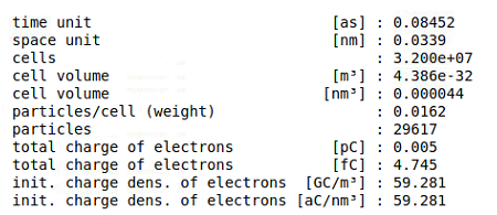
But my definition for weight is cellVolume * BASE_DENSITY with BASE_DENSITY = 3.7e+29; # [atoms/m^3]

[PrometheusPi]

@cbontoiu Okay, your minimal weighting looks very good. Thus I am still confused where the artifacts come from. Especially the pixelate substructure looks strange.
How large is the x-spacing of your density compared to the x-cell width and how do you initialize you 6ppc (random or quite)? Some intrinsic noise might come from the in-cell particle distribution. If you chose random, the position inside the cell is random. But since the density is calculated based on the macro-particle shape, these random positions might have a contribution to neighboring cells and thus might cause this pixilated noise. This could be avoided by using more ppc (and/or quickly checked by switching to a quite start).

[cbontoiu]

@PrometheusPi
The layer thickness is 0.1 nm thick and the transverse mesh size is 0.034 nm. The distance between layers is 0.34 nm so the resolution should be fine. Maybe it should be increased a bit to have let's say more than five cells per layer thickness instrad of ~3 as it is the fcase now?

My speciesInitialization.param file contains

and my particle.param file contains

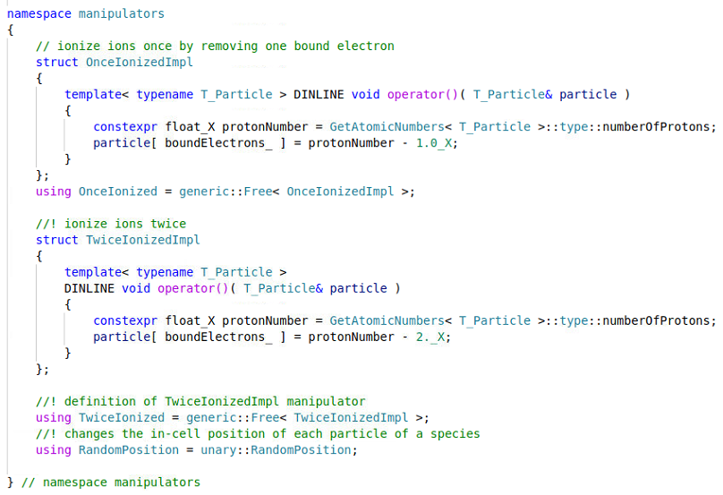
and

So I assume there is some randomization of particles at start. On the other hand I don't know what "a quite start" means. Maybe you could porive an example so I can compare the output? Thank you

[PrometheusPi]

@cbontoiu Thanks for the update.

Yes, you are using a "random" start. An example of a "quiet" start can be found in der Kelvin Helmholtz example with the according speciesInitialization.param and the particle.param(with the quite definition).

3 sample points per density layer seems to be quite low. Even though I have never played around with these strong fluctuations at the resolution limit, I would assume they effect the field solver significantly since your current is thus badly sampled. (But this does not explain your noise you see.) I would go for at least 10 cells per layer, better 20.

If you only use 3 cells per layer and use the default particle shape TSC your assignment function spans 3 cells. Thus the density you plot is influenced by the macro particles everywhere, even in the vacuum gaps.

[cbontoiu]

@PrometheusPi and @sbastrakov

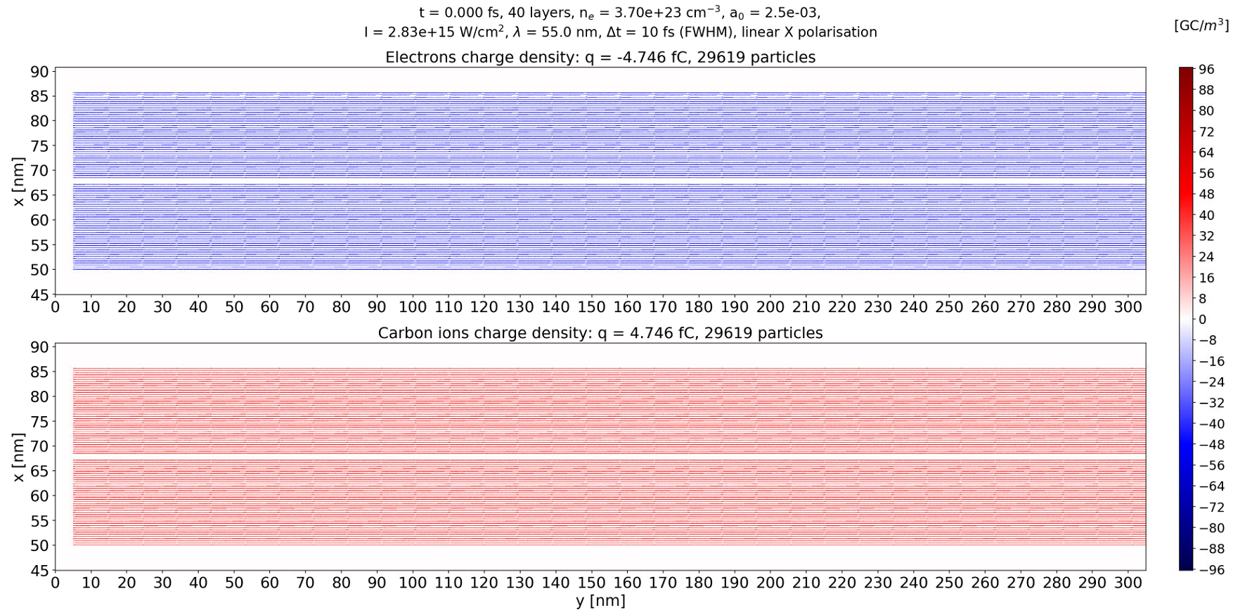
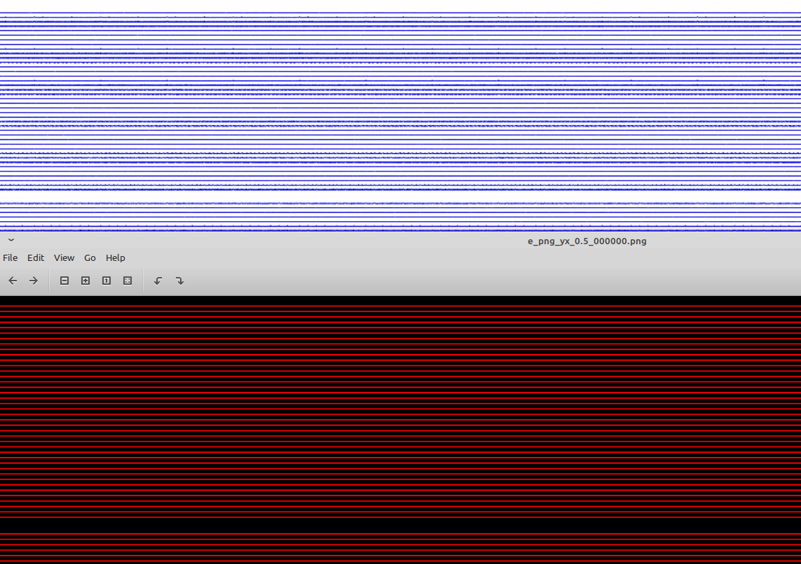
Hello on this problem once again. I am confused by the fact that particle density written as 1MB png image with namespace preParticleDensCol = colorScales::red; seems perfectly sharp at t = 0 (bottom snapshot) while mine (top snapshot) also ~1MB in size shows artifacts. This is probably due to matplotlib/python rendering but I have two questions:

1. Does anyone know a trick to improve rendering? My code looks like this

def get_electronsCharge(series, iteration, coord=io.Mesh_Record_Component.SCALAR):
    it = series.iterations[iteration]
    mesh = it.meshes['e_chargeDensity']
    component = mesh[coord]
    data = component[()] * component.unit_SI
    factor = component.unit_SI;
    return data, factor;
class MidpointNormalize(mpl.colors.Normalize):
    def __init__(self, vmin, vmax, midpoint=0, clip=False):
        self.midpoint = midpoint
        mpl.colors.Normalize.__init__(self, vmin, vmax, clip)

    def __call__(self, value, clip=None):
        normalized_min = max(0, 1 / 2 * (1 - abs((self.midpoint - self.vmin) / (self.midpoint - self.vmax))))
        normalized_max = min(1, 1 / 2 * (1 + abs((self.vmax - self.midpoint) / (self.midpoint - self.vmin))))
        normalized_mid = 0.5
        x, y = [self.vmin, self.midpoint, self.vmax], [normalized_min, normalized_mid, normalized_max]
        return sp.ma.masked_array(sp.interp(value, x, y))

        value1, factor = get_electronsCharge(ts, it);
        ts.flush();
        def function1(x, y): 
                return value1[y, x] * factor*1e-9; # in GC/m^3 
        quantity1 = function1(X, Y); 
        quantity1 = quantity1[:-1, :-1]; 
        tc = uXspace * uYspace * uZspace * value1.sum() * factor;
        chargeElectrons = str("{0:.3f}".format(tc*1e15)); # in fC
        numberElectrons = str(int(-tc/e)); 

extremes = []; extremes.append(abs(quantity1.min())); 
extremes.append(abs(quantity1.max()));
extremes.append(abs(quantity2.min())); 
extremes.append(abs(quantity2.max()));
lim = max(extremes);
levels1 = MaxNLocator(nbins=NN).tick_values(-lim, lim); 
norm1 = MidpointNormalize(vmin=-lim, vmax=lim, midpoint=0)
axes.flat[0].set_title("Electrons charge density: q = " + chargeElectrons + " fC, " + numberElectrons + " particles", fontsize = sz)
im = axes.flat[0].pcolormesh(Y*uYspace*1e9, X*uXspace*1e9, quantity1, cmap=cmap, norm=norm1, vmin = -lim, vmax= lim, rasterized=True)
cb = fig.colorbar(im, ax=axes.flat, aspect=55)
cb.ax.tick_params(labelsize = cbFS)
cb.set_label('[GC/$m^3$]', fontsize = lFS, rotation = 0, horizontalalignment='right', y=legYPos);
tick_locator = ticker.MaxNLocator(nbins=NNbar); 
cb.locator = tick_locator; 
cb.update_ticks();
fig.savefig(destinationFolder + figName, bbox_inches='tight', dpi=2*res);
plt.close(fig);

1. Is there a way to obtain the source data (maybe as text files) for the PIConGPU png images, at the runtime. something happens with the 'e_chargeDensity' field when it is being un/bundled through ADIOS. One idea is to extract charge density information from the PIConGPU images using some image processing software but that would be silly and tricky.

Any help is greatly appreciated.
Thank you.
Cristian

[sbastrakov]

Hello @cbontoiu .

Not sure how useful, but here is what I've found.
There seems to be no easy (= without or with just an obvious code modification) way to output the contents of a .png in the text form.
While looking at the code making the PNGs, the particle density is computed based on the centers of macroparticles only, so from the shapes point of view for the zero-order shape. That probably explains the sharp borders. The PIConGPU charge density for the hdf5/adios output is however computed using the actual shapes, with each macroparticle contributing to a few neighbor cells, which makes it look more smooth. And this is the actual simulation charge density that the code "sees", e.g. indirectly as part of current deposition.

[PrometheusPi]

@cbontoiu The macro-particle shape that @sbastrakov mentioned might indeed cause your hdf5/adios files in python to looks smeared out. You could avoid this by applying a particle pinning directly on a grid with bins equivalent to your cells using np.histogram2d on the particles' possitionOffset data.