Vedo: Plotly 3d vedo equivalent

[edmontz]

After familiarizing myself with the python plotly module, I find that the rendering
is rather slow; especially for iso volumes.
To evaluate this I shall include some code, the effect becomes more apparent
as the value of n, a power of two in this instance, is increased.

Perhaps you're able to provide the equivalent code using vedo, then I might
make a comparison; this will also add to your examples.

If possible, a render to screen, rather than the web browser, as this may be faster; though this may also be sent to a web page through some vedo code
that I'm not familiar with.

#   Three volume plots ; using subplots.
#   Some from a 3d array .
#   Now using 3d array and fftn, fftshift, ifftn .

import plotly.offline as py  # attempting to speed up render.

import plotly.graph_objects as go
from plotly.subplots import make_subplots

import numpy as np
from scipy.fftpack import fftn, ifftn, fftshift
import scipy.signal as sg

# ------------------------------------------------------------------

# np.ndarray(shape=(2,2), dtype=float, order='F')

n=64
m=n
p=n

# arr = np.ndarray(shape=(n,m,p), dtype=float)
# Generate data
p1=p
m1=m
n1=n
p1=int(p1/4)
m1=int(m1/9)
n1=int(n1/5)

X, Y, Z = np.mgrid[:n, :m, :p]
vol = np.zeros((n, m, p))


x1=X.flatten()
y1=Y.flatten()
z1=Z.flatten()




for k in range(p1):
    for j in range(m1):
        for i in range(n1):
            vol[i,j,k]=1
            #vol[i,j,k]=k*m1*n1 + j*n1 + i

# ------------------------------


vol /= vol.max()

volf = fftn(vol) # spectra .
volg = volf # unaltered, for further processes, possibly ifftn .
# other code here  .

volg = ifftn(volg)
volg = volg.real

# Preprocess spectra before 3d graph .

volf = abs(volf)
volf = fftshift(volf) # for centered spectra.
volf /= volf.max()
Ag=10^6
volf = np.log(Ag*volf +1)/np.log(Ag+1) # to bring out detail .


# ------------------------- Graphing results ---------------------------
# Make figure with subplots

fig = make_subplots(
    rows=3, cols=1,
    specs=[[{'type': 'Volume'}], [{'type': 'Volume'}],
           [{'type': 'Volume'}]])

# Initialize figure with 3 3D subplots


#subplot_titles=("data 3d", "3d log|fft|", "3d Real(ifft)")       
          # )


# ------------------------------------------------------------------

# adding volumes to subplots.

fig.add_trace(
    go.Volume(
    x=x1,
    y=y1,
    z=z1,
    value=vol.flatten(),
    isomin=0.1,
    isomax=1.0,
    opacity=0.1, # needs to be small to see through all surfaces
    surface_count=17 # needs to be a large number for good volume rendering
    ),
    row=1, col=1
    )    


fig.add_trace(
    go.Volume(
    x=x1,
    y=y1,
    z=z1,
    value=volf.flatten(),
    isomin=0.1,
    isomax=1.0,
    opacity=0.1, # needs to be small to see through all surfaces
    surface_count=17 # needs to be a large number for good volume rendering
    ),
    row=2, col=1
    )

fig.add_trace(
    go.Volume(
    x=x1,
    y=y1,
    z=z1,
    value=volg.flatten(),
    isomin=0.1,
    isomax=1.0,
    opacity=0.1, # needs to be small to see through all surfaces
    surface_count=17 # needs to be a large number for good volume rendering
    ),
    row=3, col=1
    )


fig.update_layout(
    title_text='3D subplots with different colorscales',
    height=1800,
    width=1024
)

#fig.show()
# plot offline

py.plot(fig, filename='isosurface.html')

# ------------------------------------------------------------------

quit()

[marcomusy]

well this takes <1s to run and render:

import numpy as np
from scipy.fftpack import fftn, ifftn, fftshift

n=64
m=n
p=n

# Generate data
p1=p
m1=m
n1=n
p1=int(p1/4)
m1=int(m1/9)
n1=int(n1/5)

X, Y, Z = np.mgrid[:n, :m, :p]
vol = np.zeros((n, m, p))

for k in range(p1):
    for j in range(m1):
        for i in range(n1):
            vol[i,j,k]=1

vol /= vol.max()

volf = fftn(vol) # spectra .
volg = volf # unaltered, for further processes, possibly ifftn .

volg = ifftn(volg)
volg = volg.real

# Preprocess spectra before 3d graph .
volf = abs(volf)
volf = fftshift(volf) # for centered spectra.
volf /= volf.max()
Ag=10^6
volf = np.log(Ag*volf +1)/np.log(Ag+1) # to bring out detail .

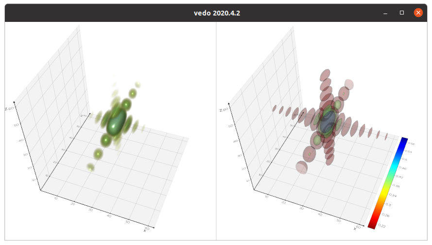
from vedo import Volume, show
v = Volume(volf).printInfo()
isos = v.isosurface([0.2,0.4,0.6]).alpha(0.2).addScalarBar3D()
show(v, isos, N=2, axes=1)

[edmontz]

I had to comment out the .addScalarBar3D() to get this to work, perhaps I need
to upgrade my version of vedo; presently at 2020.4.0 ? This might be an issue
with my GPU.
How slow was my original code on your computer, I used 17 levels for the
iso surface in that instance.
On my computer your code renders in a few seconds.
For some reason the two 3d graphs have different sized viewports, maybe
as in plotly there's some way to predefine the limits.

With n from 32 through 256, all of your code functions, beyond that, at 512,
my portion of the code quits.

[marcomusy]

I had to comment out the .addScalarBar3D() to get this to work, perhaps I need
to upgrade my version of vedo; presently at 2020.4.0 ? This might be an issue
with my GPU.

Try with
pip install -U git+https://github.com/marcomusy/vedo.git

How slow was my original code on your computer, I used 17 levels for the
iso surface in that instance.

very slow:)

With n from 32 through 256, all of your code functions, beyond that, at 512,
my portion of the code quits.

you might have hit some memory limit.

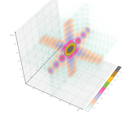
PS : another intersting rendering option is with _max projection_ (instead of _composite_ mode):

Volume(volf).mode(1).c('Dark2').alpha([0,0.8,1]).addScalarBar3D().show(axes=1)

[edmontz]

I upgraded to 4.1 and was then able to include the scalar bar, though for large
values of n I commented this out again also I set axes=0 .

Firstly do this #X, Y, Z = np.mgrid[:n, :m, :p] , comment out the grid creation, it
isn't required for the way I'm generating data. I found the plot to be much more
responsive.

After that I was able to set n to 512, after less than a minute this also rendered, however zooming or rotating was rather slow.

Volume(volf).mode(1).c('Dark2').alpha([0,0.8,1]).addScalarBar3D().show(axes=1)

Is valid on my computer, for n = 512, also the render is quite responsive to zoom and rotation. There are no issues with the axes or scalarbar either.

I'd been using show(v, isos, axes=0) .

[edmontz]

I posted more code at the website; this you replied to..

Beyond that I have two more questions..

To draw three distinct volumes I'm using:

from vedo import Volume, show

va = Volume(vol).mode(1).c('winter').alpha([0,0.6,0.8,1])
vb = Volume(volf).mode(1).c('winter').alpha([0,0.6,0.8,1])
vc = Volume(volg).mode(1).c('winter').alpha([0,0.4,0.6,0.8,1]).addScalarBar3D()

show([va,vb,vc], shape=[1,3], axes=1,bg='black')

Is there a way to graph the three volumes without using the Volume() routine.

And, off topic, are you familiar with scipy

[marcomusy]

I posted more code at the website;

which website?

Is there a way to graph the three volumes without using the Volume() routine.

Not sure what you mean. Your volf etc, are numpy arrays.

And, off topic, are you familiar with scipy

Yes :) but please understand that I can only offer support to vedo.

[edmontz]

This website.

Previously we used

Volume(volf).mode(1).c('Dark2').alpha([0,0.8,1]).addScalarBar3D().show(axes=1)

to directly graph a single 3d numpy array. Is it possible to use this with more 3d numpy arrays within the same command. Does this command generate other
arrays prior to plotting.

[marcomusy]

Is it possible to use this with more 3d numpy arrays within the same command

..no, each numpy array is used to create a separate object of class vedo.Volume

Does this command generate other arrays prior to plotting.

no it doesn't

[edmontz]

Does tk do most of the graphics computation.

For basic, interactive, animation this is what I have produced.

#
#   Iterated volume plots from 3d array.
# 



import numpy as np
from scipy.fftpack import fftn, ifftn, fftshift
import scipy.signal as sg


from vedo import Volume, show

from vedo import *

# ---------------------- functions -------------------------------------

def f3(x,y,z,t):
    #r=x*x+y*y+z*z+t*t*2
    #r=np.sqrt(r) + 0.01
    #w=np.sin(r*np.pi*9)/r
    r=np.pi*3*t
    w=np.sin(r*x*7+y)*cos(r*y*5+sin(3*z*r)*r)*sin(r*z*3+x)

    return w


# ------------------------------------------------------------------



vp = Plotter(interactive=0, axes=0)


# ------------------------------------------------------------------

# np.ndarray(shape=(2,2), dtype=float, order='F')

n=64
m=n
p=n

n1=n
m1=m
p1=p

n1=int(n1/2)
m1=int(m1/2)
p1=int(p1/2)
# Use a mesh ?

# X,Y,Z=np.mesh([],[],[])


Ag=10^6
Pd=np.log(Ag+1)
vol = np.zeros((n, m, p))

#pb = ProgressBar(0, 100, c="r")
qn=100
for q in range(qn):

    t=2*q/qn -1
    for k in range(p1):
        z=2*k/p1 - 1
        for j in range(m1):
            y=2*j/m1-1
            for i in range(n1):
                x=2*i/n1-1
                vol[i,j,k]=f3(x,y,z,t)

    volf = fftn(vol)
    volf = abs(volf)
    volf = fftshift(volf) # for centered spectra
    volf /= volf.max()

    volf = np.log(Ag*volf +1)/Pd # to bring out detail .
    vb = Volume(volf).mode(1).c('rainbow').alpha([0,0.8,1])
    vp.show(vb, axes=0,bg='black')

vp.show(interactive=1)  


quit()

[marcomusy]

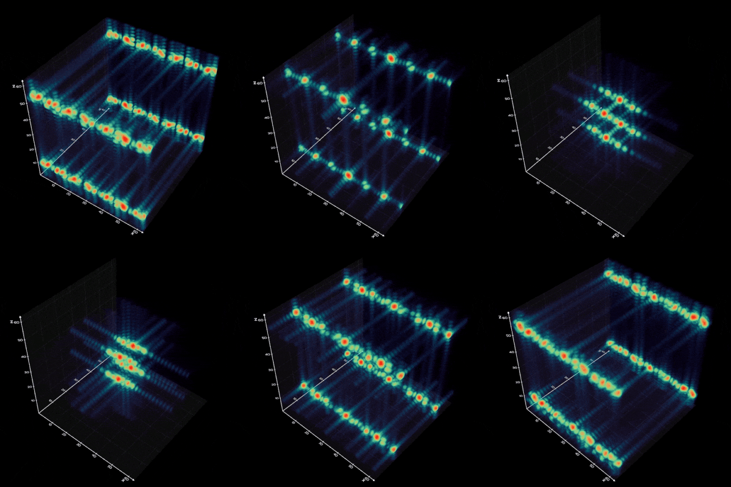
looks cool :)
maybe adding axes gives it some better intuition of depth:

import numpy as np
from scipy.fftpack import fftn, fftshift
from vedo import Volume, show, interactive, sin, cos, ProgressBar, Video

def f3(x, y, z, t):
    # r=x*x+y*y+z*z+t*t*2
    # r=np.sqrt(r) + 0.01
    # w=np.sin(r*np.pi*9)/r
    r = np.pi*3*t
    w=np.sin(r*x*7+y)*cos(r*y*5+sin(3*z*r)*r)*sin(r*z*3+x)
    return w

n = 64
m = n
p = n

n1 = n
m1 = m
p1 = p

n1 = int(n1 / 2)
m1 = int(m1 / 2)
p1 = int(p1 / 2)

Ag = 10 ^ 6
Pd = np.log(Ag + 1)
vol = np.zeros((n, m, p))

qn = 100
vd = Video(duration=5, backend='cv')
pb = ProgressBar(0, qn, c="r")
for q in pb.range():
    pb.print()

    t = 2 * q / qn - 1
    for k in range(p1):
        z = 2 * k / p1 - 1
        for j in range(m1):
            y = 2 * j / m1 - 1
            for i in range(n1):
                x = 2 * i / n1 - 1
                vol[i, j, k] = f3(x, y, z, t)

    volf = fftn(vol)
    volf = abs(volf)
    volf = fftshift(volf)  # for centered spectra
    volf /= volf.max()

    volf = np.log(Ag * volf + 1) / Pd  # to bring out detail
    vb = Volume(volf).mode(1).c("rainbow").alpha([0, 0.8, 1])
    show(vb, bg="black", axes=1, viewup='z', azimuth=.1, interactive=0)
    vd.addFrame()

vd.close()
interactive()

PS: note that 10^6 = 12 in python

[edmontz]

With axes=1 I effectively reproduce what you have shown.

I also manage to generate a file called movie.mp4, however I am unable to view that in my Firefox
browser.
How did you produce the above video ; looks like you made an animated gif .

[edmontz]

Now this is puzzling; I can not animate two graphs at the same time.

Also, I notice that your code has syntax colouring, is this an option within this comments box.

import numpy as np
from scipy.fftpack import fftn, fftshift
from vedo import Volume, show, interactive, sin, cos, ProgressBar, Video

def f3(x, y, z, t):
    # r=x*x+y*y+z*z+t*t*2
    # r=np.sqrt(r) + 0.01
    # w=np.sin(r*np.pi*9)/r
    r = np.pi*3*t
    w=np.sin(r*x*7+y)*cos(r*y*5+sin(3*z*r)*r)*sin(r*z*3+x)
    return w

n = 64
m = n
p = n

n1 = n
m1 = m
p1 = p

n1 = int(n1 / 2)
m1 = int(m1 / 2)
p1 = int(p1 / 2)

# Python power, choose colormap carefully when using this. 
#Ag = 10 ** 6


Ag = 10
Pd = np.log(Ag + 1)
vol = np.zeros((n, m, p))

qn = 100
vd = Video(duration=5, backend='cv')
pb = ProgressBar(0, qn, c="r")
for q in pb.range():
    pb.print()

    t = 2 * q / qn - 1
    for k in range(p1):
        z = 2 * k / p1 - 1
        for j in range(m1):
            y = 2 * j / m1 - 1
            for i in range(n1):
                x = 2 * i / n1 - 1
                vol[i, j, k] = f3(x, y, z, t)

    volf = fftn(vol)
    volf = abs(volf)
    volf = fftshift(volf)  # for centered spectra
    volf /= volf.max()

    volf = np.log(Ag * volf + 1) / Pd  # to bring out detail
    vb = Volume(volf).mode(1).c("rainbow").alpha([0, 0.8, 1])

    vol /= vol.max()
    va = Volume(vol).mode(1).c("winter").alpha([0, 0.1,0.4,0.8, 1])

    show([va,vb],shape=[1,2], bg="black", axes=1, viewup='z', azimuth=.1, interactive=0)
    vd.addFrame()

vd.close()
interactive()

#
# To convert mp4 video to animated gif , from terminal.
#
# ffmpeg -i movie.mp4 fft3da.gif
#
#
# Generally use this type of command.
#
# ffmpeg -i input_video_file output.gif

[marcomusy]

to have syntax coloring use:

to make gif from videos I use: https://ezgif.com/video-to-gif

I can not animate two graphs at the same time.

This is actually a limitation/bug in vedo syntax which is not very intuitive and should be improved. This should work:

    show(va, at=0, shape=[1,2], bg="black", axes=1, viewup='z')
    show(vb, at=1, bg="black", axes=1)

[edmontz]

A few improvements to the previous code.

In an attempt to speed up the calculations, via numba, I restructed
the program and seperated the code into functions.

Not all of these functions were able to be sped up, in particular the
main function, with calls to scipy fft routines; couldn't be.
Nevertheless, I was expecting greater than a 2 times improvement as the
numba speed up for the compiled functions was 100x, or more.

The fft package from scipy, contains a number of features that are
difficult to emulate in any version I might construct.

#      Speed up with numba , except for fftn ; not supported in numba.
#      If we're only interested in the standard radix 2 fft, then write
#     your own code and compile with jit ?
#      Timing  , call function once to compile; again when already compiled. 


from vedo import Volume, show, interactive, sin, cos, ProgressBar, Video


from numba import jit
import numpy as np
import time

from scipy.fft import fftn,fftshift

# n = 32, 64, 128, 256, 512

n = 128
m = n
p = n

n1 = n
m1 = m
p1 = p

n1 = int(n1 / 2)
m1 = int(m1 / 2)
p1 = int(p1 / 2)

# -----------------

vol = np.zeros((n, m, p),dtype=np.float32)
x=0.0
y=0.0
z=0.0
t=0.0

@jit(nopython=True)
def f32(x, y, z, t)->np.float32:
    r = np.pi*3*t
    w = np.sin(r*x*7+y*r)*np.cos(r*y*5+np.sin(3*z*r)*r)*np.sin(r*z*3+x*r) + 0.0000001
    #r = np.pi*5*t
    #r = np.sqrt(x*x + y*y + z*z)*r
    #w = (np.sin(r)+0.01)/(r+ 0.01)
    w = np.log(100*abs(w) + 1)
    return w

@jit(nopython=True)
def genf2(vol: np.float32,n1: int,m1: int,p1: int,t :np.float32):

    for k in range(p1):
        z= (-1+(2*k/p1))

        for j in range(m1):
            y= (-1+(2*j/m1))
            for i in range(n1):
                x= (-1+(2*i/n1))
                vol[i,j,k] = f32(x,y,z,t)


    return vol              


@jit(nopython=True)
def fnvol(volf: np.float32):
    Ag = 100
    Pd = np.log(Ag + 1)
    volf = np.abs(volf)
    vm = volf.max()
    vm = np.abs(vm)
    if (vm > 0.0 ):
        volf = volf/vm
    volf = np.log(Ag*volf + 1)/Pd

    return volf


#w=f32(x,y,z,t)
#vol=genf2(vol,n1,m1,p1,t)


# ----------------------------------------------------
# qn = 100 , duration=6 , fps ~= 15
# fps ~= qn/duration
# =>  duration = qn/fps

qn=500 # number of frames.
fps=30 # frames per second
vidlen=qn/fps # video length, in seconds 
print(" length of video, in seconds")
print(vidlen)
vd = Video(duration=vidlen, backend='cv')

# @jit
def main(vol,vd,qn):
    #qn = 100
    #vd = Video(duration=6, backend='cv')
    #pb = ProgressBar(0, qn, c="r")
    #q=int(0)
    for q in range(0,qn,1):
        t = (2 * q / qn) - 1
        vol = genf2(vol,n1,m1,p1,t)
        volf = fftn(vol)
        volf = fftshift(volf)
        volf = fnvol(volf)
        vb = Volume(volf).mode(1).c("rainbow").alpha([0, 0.8, 1])
        vm = np.abs(vol.max())
        if (vm>0):
            vol = vol/vm
        va = Volume(vol).mode(1).c("gist_rainbow").alpha([0, 0.1,0.4,0.8, 1])
        show(va, at=0, shape=[1,2], bg="black", axes=1, viewup='z')
        show(vb, at=1, bg="black", axes=1)
        vd.addFrame()

start = time.time()
main(vol,vd,qn)
end = time.time()



vd.close()
interactive()

# Typical times, in seconds, for original f32().

# 60.743521213531494   python  ,                    n = 64

# 21.xx                numba , without frame save , n = 64 .
# 32.16198372840881    numba ,                      n = 64

# 39.6319305896759     numba , without frame save , n = 128
# 52.91490864753723    numba ,                      n = 128

# 195.10343718528748   numba , without frame save , n = 256
# 231.9945890903473    numba ,                      n = 256

#    numba , without frame save , n = 512
#    numba ,                      n = 512


print("Elapsed (with compilation) = %s" % (end - start))

quit()

[edmontz]

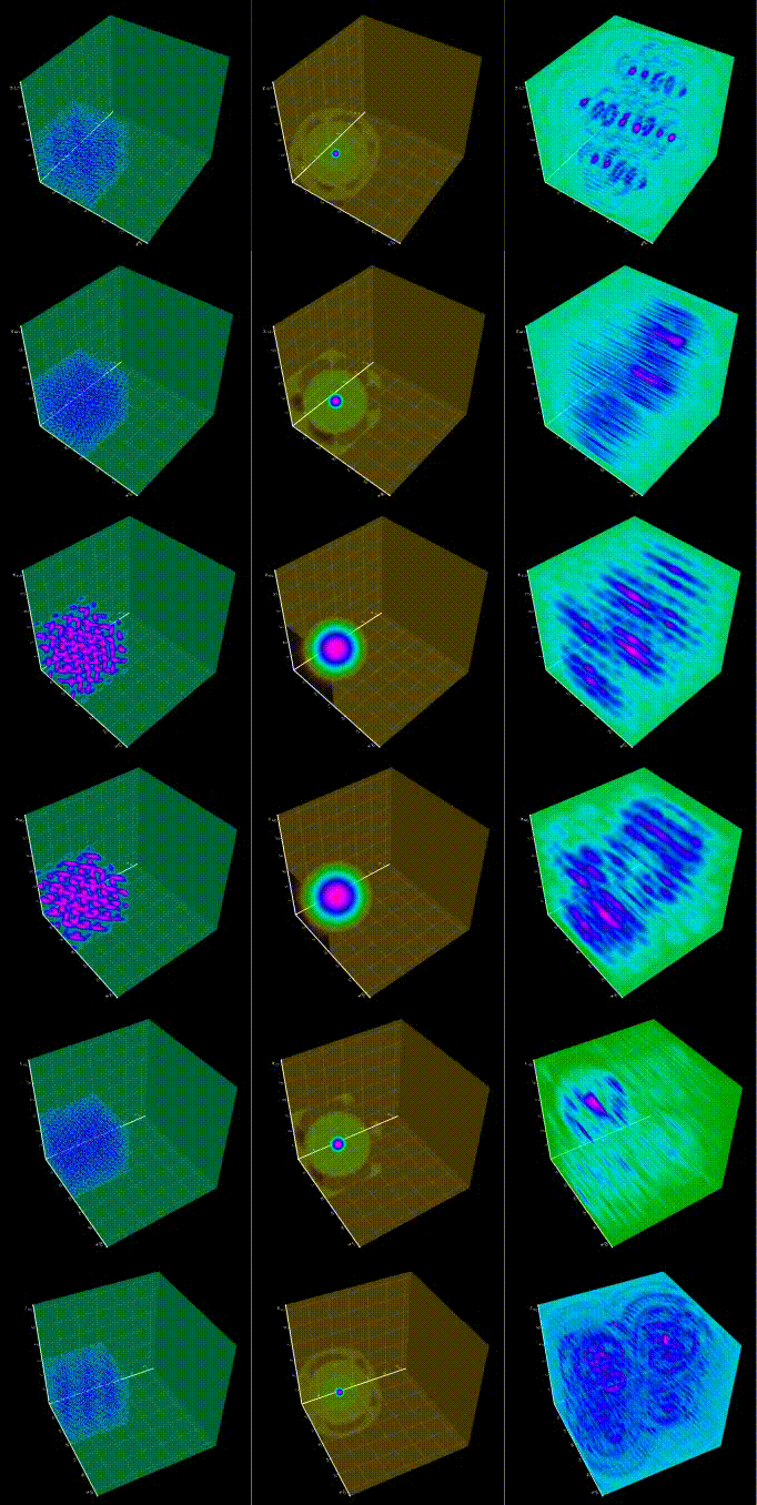
Introducing 3d convolution .

```python

3d convolution via fft

The inputs and output also include negative values.

Speed up with numba , except for fftn ; not supported in numba.

If we're only interested in the standard radix 2 fft, then write

your own code and compile with jit ?

Timing , call function once to compile; again when already compiled.

from vedo import Volume, show, interactive, sin, cos, ProgressBar, Video

from numba import jit
import numpy as np
import time

from scipy.fft import fftn,fftshift, ifftn

n = 32, 64, 128, 256, 512

n = 64
m = n
p = n

n1 = n
m1 = m
p1 = p

n1 = int(n1 / 2)
m1 = int(m1 / 2)
p1 = int(p1 / 2)

-----------------

vol = np.zeros((n, m, p),dtype=np.float32)
vol1 = np.zeros((n, m, p),dtype=np.float32)

x=0.0
y=0.0
z=0.0
t=0.0

def convn(a1,b1):
# Restrict data to the first half, then similar to mode = 'same' ?.
# a1 and b1 real, easily updated to complex.

A1=fftn(a1)
B1=fftn(b1)
C1=np.multiply(A1,B1)
c1=ifftn(C1)
c1=c1.real
return c1

@jit(nopython=True)
def f31(x, y, z, t)->np.float32:
r = np.pi5t
r = np.sqrt(xx + yy + zz)r
w = (np.sin(r)+0.01)/(r+ 0.01)
return w

@jit(nopython=True)
def f32(x, y, z, t)->np.float32:
r = np.pi3t
w = np.sin(rx7+yr)np.cos(ry5+np.sin(3zr)r)np.sin(rz3+x*r) + 0.0000001

return w

@jit(nopython=True)
def genf1(vol1: np.float32,n1: int,m1: int,p1: int,t :np.float32):

for k in range(p1):
    z= (-1+(2*k/p1))

    for j in range(m1):
        y= (-1+(2*j/m1))
        for i in range(n1):
            x= (-1+(2*i/n1))
            vol1[i,j,k] = f31(x,y,z,t)


return vol1

@jit(nopython=True)
def genf2(vol: np.float32,n1: int,m1: int,p1: int,t :np.float32):

for k in range(p1):
    z= (-1+(2*k/p1))

    for j in range(m1):
        y= (-1+(2*j/m1))
        for i in range(n1):
            x= (-1+(2*i/n1))
            vol[i,j,k] = f32(x,y,z,t)


return vol

@jit(nopython=True)
def fnvol1(vol1: np.float32):
vm = np.abs(vol1.max())
if (vm>0):
vol1 = vol1/vm
return vol1

@jit(nopython=True)
def fnvol(vol: np.float32):
vm = np.abs(vol.max())
if (vm>0):
vol = vol/vm
return vol

@jit(nopython=True)
def fnvolf(volf: np.float32):

vm = np.abs(volf.max())

if (vm > 0.0 ):
    volf = volf/vm


return volf

@jit(nopython=True)
def fnvolL(volf: np.float32):
# Return logarithm of scaled volf .
Ag = 100
Pd = np.log(Ag + 1)
volf = np.abs(volf)
vm = volf.max()

if (vm > 0.0 ):
    volf = volf/vm
volf = np.log(Ag*volf + 1)/Pd

return volf

----------------------------------------------------

qn = 100 , duration=6 , fps ~= 15

fps ~= qn/duration

=> duration = qn/fps

qn=100 # number of frames.
fps=30 # frames per second
vidlen=qn/fps # video length, in seconds
print(" length of video, in seconds")
print(vidlen)
vd = Video(duration=vidlen, backend='cv')

@jit

def main(vol,vol1,vd,qn):

for q in range(0,qn,1):
    t = (2 * q / qn) - 1
    vol1 = genf1(vol1,n1,m1,p1,t)   
    vol = genf2(vol,n1,m1,p1,t)

    volf = convn(vol1,vol) 
    volf = fnvolf(volf)
    vol1 = fnvol1(vol1)
    vol = fnvol(vol)

    va = Volume(vol).mode(1).c("gist_rainbow").alpha([0, 0.1,0.4,0.8, 1])
    vb = Volume(vol1).mode(1).c("gist_rainbow").alpha([0, 0.8, 1])
    vc = Volume(volf).mode(1).c("gist_rainbow").alpha([0, 0.8, 1])
    show(va, at=0, shape=[1,3], bg="black", axes=1, viewup='z', azimuth=.1, interactive=0)
    show(vb, at=1, bg="black",  axes=1, viewup='z', azimuth=.1, interactive=0)
    show(vc, at=2, bg="black",  axes=1, viewup='z', azimuth=.1, interactive=0)

    vd.addFrame()

start = time.time()
main(vol,vol1,vd,qn)
end = time.time()

vd.close()
interactive()

This took about 42 s, and rendered to the screen fairly promptly.

print("Elapsed (with compilation) = %s" % (end - start))

quit()

'''
!

[edmontz]

You don't need to import numba to run the last few examples, if you don't then comment
out all instances of the @jit function decorator. Bound to run slower after this.

Calls to fft routines use 10% of the process time, vedo appears to use most of the rest.