Prophet: Local and Server forecast results are different

[ontheroad87]

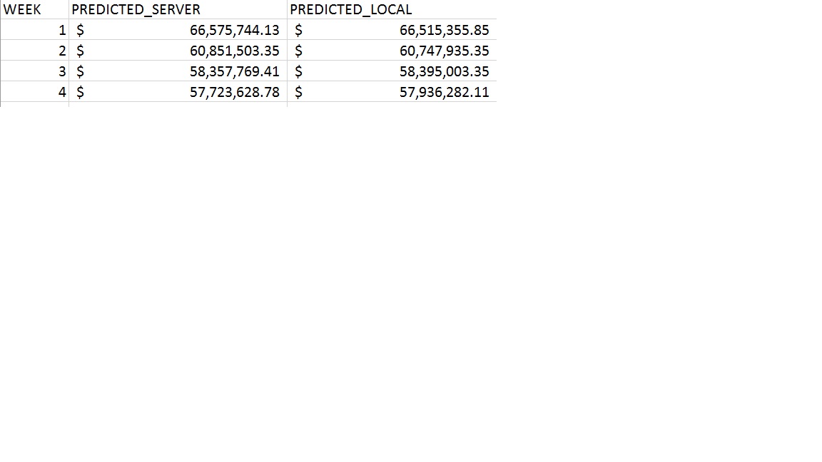
I used prophet package to make weekly forecast. I ran my code in R in my computer and on R server. The forecast results are slightly different. See code below:

m <- prophet(data,holidays = holidays,weekly.seasonality = TRUE)
future <- make_future_dataframe(m, periods = 52,freq='week')
forecast_pro <- predict(m, future)

Part of the results comparison is attached.

I also checked machine’s precision and found only sizeof.long is different. $sizeof.long is 4 in my computer and is 8 in server. Could this difference make the forecast results different? If not, is there any other reason that can make the results different?

[maskani-moh]

@ontheroad87

Don't forget that in the underlying model there is an additive noise which is random (_white noise_).

Take a closer look here. This noise is also scaled by self.y_scale, which can give more or less noticeable differences.

There are also other sources of randomness in the code.

The results might then be a little bit different if the seed is not identical in your cases.

If you need further explanations just let me know 😉

[mucun1988]

@ontheroad87 @maskani-moh also the change points in the future are also generated randomly

[maskani-moh]

@mucun1988

Yes, that is what I meant by:

There are also other sources of randomness in the code.

[ontheroad87]

Thanks for your comments! I understand the randomness in the code, but why can I always get same results in my local computer even if I run the code multiple times? Only when I run it on the server, I got different results.

[bletham]

The main yhat estimate without MCMC (default) is fairly deterministic since it uses the best-fit (maximum a posteriori) parameters. In particular, the additive noise part of the model is reflected in the log-likelihood function, but does not add randomness to the maximizer of the log-likelihood. y.scale is computed from the input data and so will be the same each run. Changepoints in the future are randomly generated for estimating trend uncertainty, but the main yhat estimate just projects forward the trend of the last segment*. The best-fit parameters are found using the L-BFGS algorithm, using a deterministic initialization. So, variance in the predictions should be coming from variance in the best-fit parameters being found by L-BFGS. I don't believe there is any actual randomness in this algorithm, but it seems plausible to me that things like machine precision could be affecting the termination conditions. This could especially be the case if the log-likelihood surface is fairly flat near the optimum (parameters are not well identified). Different versions of Stan might also do different things here.

Could you compare m$params on each of them and see where they are different?

• For the piecewise linear trend, because the trend shifts are symmetrically up or down, the expected value of all of the future trend shifts is 0, and so that process is just used to get some estimate of the variance of the future trend.

[maskani-moh]

Thanks for the feedback @bletham !

[ontheroad87]

@maskani-moh @mucun1988 @bletham

Thanks for your feedbacks! I checked the parameters. It seems that all parameters are a little bit different.
Parameters from server:
$k
[1] 0.07491082

$m
[1] -0.07294964

$delta
[,1] [,2] [,3] [,4] [,5]
[1,] 1.085872e-08 3.902014e-09 7.325707e-10 6.723302e-09 -1.572364e-09
[,6] [,7] [,8] [,9] [,10]
[1,] 1.753316e-09 4.222645e-10 1.503281e-06 0.0008669452 2.393173e-05
[,11] [,12] [,13] [,14] [,15] [,16]
[1,] 0.003931978 0.004039215 0.0174029 0.01641545 0.002849446 0.01237765
[,17] [,18] [,19] [,20] [,21]
[1,] 0.000368546 1.794284e-06 3.265981e-06 4.535584e-07 2.339677e-09
[,22] [,23] [,24] [,25]
[1,] 9.778378e-09 -3.503411e-09 7.012594e-10 5.26422e-09

$sigma_obs
[1] 0.2240761

$beta
[,1] [,2] [,3] [,4] [,5] [,6] [,7]
[1,] 0 -0.01070402 -0.05633083 -0.02373534 -0.01446308 0.01232427 0.04661591
[,8] [,9] [,10] [,11] [,12] [,13]
[1,] -0.03419499 -0.02337984 -0.04925917 0.006111457 -0.02754168 0.04966174
[,14] [,15] [,16] [,17] [,18] [,19]
[1,] -0.03421035 0.03449416 -0.01326152 -0.009835812 -0.03126241 0.005581021
[,20] [,21] [,22] [,23] [,24] [,25]
[1,] -0.03482755 0.01810901 -0.06715768 -0.1394544 0.121014 0.09650542
[,26] [,27] [,28] [,29] [,30] [,31]
[1,] -0.1509019 -0.03444238 -0.2007803 0.2622081 -0.2948083 -0.4757809
[,32] [,33] [,34] [,35] [,36] [,37]
[1,] 0.08625935 -0.561027 -0.5743847 -0.04423623 -0.0741879 0.3013889

$gamma
[1] -3.465550e-10 -2.490647e-10 -7.013974e-11 -8.582939e-10 2.509092e-10
[6] -3.357414e-10 -9.433568e-11 -3.838163e-07 -2.490162e-04 -7.637785e-06
[11] -1.380375e-03 -1.546934e-03 -7.220351e-03 -7.334562e-03 -1.364097e-03
[16] -6.320500e-03 -1.999558e-04 -1.030759e-06 -1.980435e-06 -2.895053e-07
[21] -1.568081e-09 -6.865670e-09 2.571653e-09 -5.371349e-10 -4.200176e-09

Parameters from local computer:

$k
[1] 0.07859775

$m
[1] -0.073422

$delta
[,1] [,2] [,3] [,4] [,5] [,6] [,7] [,8] [,9]
[1,] 3.934741e-09 -1.933512e-09 8.087515e-10 -2.593653e-09 -1.228869e-09 1.076716e-10 9.836732e-09 2.219188e-06 1.365488e-08
[,10] [,11] [,12] [,13] [,14] [,15] [,16] [,17] [,18] [,19]
[1,] 1.472851e-06 0.003263724 0.003726447 0.01873904 0.0174806 0.004092313 0.01248047 4.547879e-05 3.014816e-05 5.135047e-09
[,20] [,21] [,22] [,23] [,24] [,25]
[1,] 6.430502e-09 3.251524e-09 4.356411e-08 1.463851e-09 1.639798e-08 2.202868e-09

$sigma_obs
[1] 0.2246792

$beta
[,1] [,2] [,3] [,4] [,5] [,6] [,7] [,8] [,9] [,10] [,11]
[1,] 0 -0.01147433 -0.05539196 -0.02533858 -0.01476522 0.0111118 0.0471288 -0.03494813 -0.02390785 -0.05035847 0.005516094
[,12] [,13] [,14] [,15] [,16] [,17] [,18] [,19] [,20] [,21]
[1,] -0.02800926 0.0500524 -0.03471274 0.03382309 -0.01335293 -0.009910826 -0.03144626 0.005274804 -0.03537529 0.01828478
[,22] [,23] [,24] [,25] [,26] [,27] [,28] [,29] [,30] [,31] [,32]
[1,] -0.06695158 -0.1390264 0.1206426 0.09620924 -0.1504388 -0.03433668 -0.2044455 0.262159 -0.2957255 -0.4769685 0.08717124
[,33] [,34] [,35] [,36] [,37]
[1,] -0.5617904 -0.5764487 -0.04431969 -0.07390789 0.3019515

$gamma
[1] -1.255768e-10 1.234157e-10 -7.743366e-11 3.311047e-10 1.960962e-10 -2.061797e-11 -2.197568e-09 -5.666012e-07
[9] -3.922146e-09 -4.700588e-07 -1.145775e-03 -1.427150e-03 -7.774708e-03 -7.810482e-03 -1.959086e-03 -6.373007e-03
[17] -2.467466e-05 -1.731916e-05 -3.113805e-09 -4.104575e-09 -2.179213e-09 -3.058757e-08 -1.074529e-09 -1.256015e-08
[25] -1.757607e-09

[bletham]

Well there's the difference! Is the version of rstan the same on both? I think it must be related to the L-BFGS termination, could you try with the Newton algorithm to see if it gives you something more consistent?

m <- prophet(data,holidays = holidays,weekly.seasonality = TRUE, algorithm = 'Newton')

[ontheroad87]

@bletham @maskani-moh @mucun1988
Yes, the version of rstan is same on both. I tried Newton algorithm and then the results are the same!!!
Thanks a lot!