Picongpu: Ionization and charge density
Hello,
I am trying to make sense of laser interaction with a carbon structure, preionized one. I have two cases:
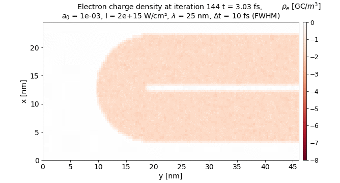
1) the wavelength is 25 nm and a0 = 1e-03 and i get a kind of standing wave; ionization progresses at the maxima of the laser Ex electric field as shown in the first gif. Is this an error? I expected the laser pulse to ionize all the way at a growing rate as the Gaussian pulse reaches the top.
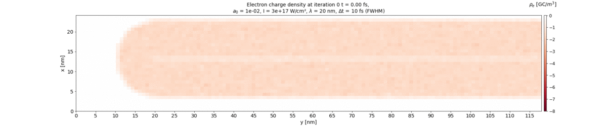
2) the wavelength is 20 nm and the a0 = 1e-2. Now I get something more related to what i expect bu at some point all electrons disappear and the same happens with the carbon ions. What am I doing wrong here?
On the other hand for the second case the default png images still show the electrons as you can see in the gif below.

Yet another situation of losing the beam is shown in the figure below
for this last one I used absorber at all 6 faces with the YeePML solver so
I don't know if it was a good idea.
I would be grateful for any suggestion.
Thank you.
 cbontoiu
All 24 comments
Dear @cbontoiu,
thank you for reporting this issue. In order to make sense of the simulation output, could you please provide the laser.param, density.paramand speciesInitalization.param (for now).
Could you also upload fields_energy.dat and e_macroParticlesCount.dat?
That would help us tremendously in understanding/guessing what happened.
The ionization you show in your first gif makes no sense to me. What ionization model did you select? Which slice did you plot? What are the electric field values during that time evolution?
 PrometheusPi
on 9 Mar 2020
PrometheusPi
on 9 Mar 2020
Thank you very much for your availability to help.
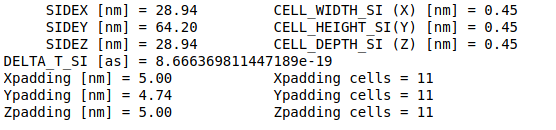
First of all I have to say that I noticed a difference between using the Yee and the YeePML solver. For the same DELTA_T_SI the first one complains about the Courant–Friedrichs–Lewy condition while the latter one accepts it. I don't know if this is something you want to keep.
I attach the whole input folder below (with YeePML). This is reduced-mesh model that can run quickly on my single GPU machine.
The model uses a PlaneWave laser as shown below.
struct PlaneWaveParam
 {
  static constexpr float_64 PULSE_LENGTH_SI = (10e-15)/2.354820045;
  static constexpr float_64 WAVE_LENGTH_SI = 20e-09;
  static constexpr float_64 _A0 = 5e-03;
  static constexpr float_64 UNITCONV_A0_to_Amplitude_SI = -2.0 * PI / WAVE_LENGTH_SI *
   ::picongpu::SI::ELECTRON_MASS_SI * ::picongpu::SI::SPEED_OF_LIGHT_SI *
   ::picongpu::SI::SPEED_OF_LIGHT_SI / ::picongpu::SI::ELECTRON_CHARGE_SI;
  static constexpr float_64 AMPLITUDE_SI = _A0 * UNITCONV_A0_to_Amplitude_SI;
  static constexpr float_64 LASER_NOFOCUS_CONSTANT_SI = 0.0;
  static constexpr float_64 RAMP_INIT = 3. * 2.354820045;
  static constexpr uint32_t initPlaneY = 0;
  static constexpr float_X LASER_PHASE = 0.0; // 3.14159265359/2;
  enum PolarisationType { LINEAR_X = 1u, LINEAR_Z = 2u, CIRCULAR = 4u };
  static constexpr PolarisationType Polarisation = LINEAR_X;
  };
The density is just a simple tube with rounded end at the left Y side
namespace densityProfiles
{
    constexpr double diamINCNT  =  1.35e-09;
    constexpr double diamOUTCNT = 18.94e-09;
    constexpr double MARGIN = 5e-09;
    constexpr double rad_in = diamINCNT/2;
    constexpr double rad_out = diamOUTCNT/2;
    constexpr double mYL = diamOUTCNT;
    struct XZTubesFunctor
    {
        double Z0 = rad_out + MARGIN;
        double X0 = rad_out + MARGIN;
        HDINLINE float_X
        operator()( const floatD_64& position_SI, const float3_64& cellSize_SI )
        {
          const float_64 z( position_SI.z() );
          const float_64 y( position_SI.y() );
          const float_64 x( position_SI.x() );
          float_64 dens = 0.0;
          // generate density for hollow tubes ...............................
          double distanceTube = (z-Z0)*(z-Z0) + (x-X0)*(x-X0);
          if( distanceTube >= rad_in*rad_in && distanceTube <= rad_out*rad_out)
              { if( y >= mYL)  dens = 1.0; }
          // generate density for hollow tubes ...............................
          double distanceEndCap = (z - Z0)*(z - Z0) + (x - X0)*(x - X0) + (y - mYL)*(y - mYL);
          if( distanceEndCap >= rad_in*rad_in && distanceEndCap <= rad_out*rad_out)
             { if( y < mYL) dens = 1.0; }
          // safety check: all parts of the function MUST be > 0
          dens *= float_64( dens >= 0.0 );
          return dens;
        }
    };
For species initialization I use 16ppc but the same problem appears for 6 ppc
using InitPipeline = bmpl::vector<
 CreateDensity< densityProfiles::XZTubes, startPosition::Random16ppc, Carbon >,
 Manipulate< manipulators::OnceIonized, Carbon >,
 ManipulateDerive< manipulators::binary::UnboundElectronsTimesWeighting, Carbon, Electrons >,
 CreateDensity< densityProfiles::ProbeEveryFourthCell, startPosition::OnePosition, Probes >
>;
The energy and macroparticles files are here
fields_energy.dat.txt
e_macroParticlesCount.dat.txt
e_energy_all.dat.txt
C_macroParticlesCount.dat.txt
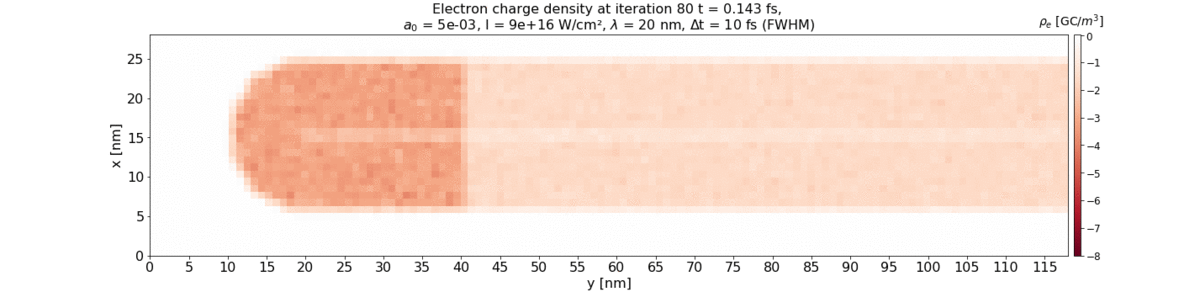
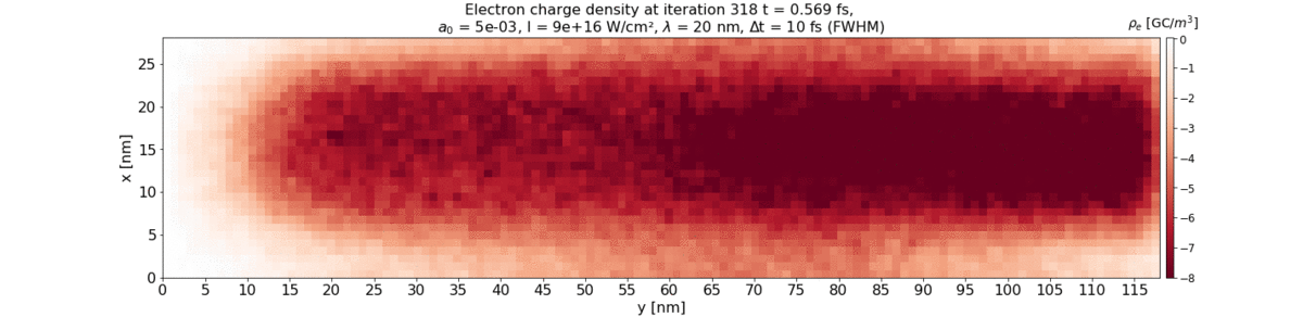
What I obtain is in the figures below (beginning and end):
About ionization, i use all three available types:
using ParticleFlagsCarbon = MakeSeq_t<
    particlePusher< UsedParticlePusher >,
    shape< UsedParticleShape >,
    interpolation< UsedField2Particle >,
    current< UsedParticleCurrentSolver >,
    massRatio< MassRatioCarbon >,
    chargeRatio< ChargeRatioCarbon >,
    densityRatio< DensityRatioCarbon >,
    atomicNumbers< ionization::atomicNumbers::Carbon_t >,
    ionizationEnergies< ionization::energies::AU::Carbon_t >,
    effectiveNuclearCharge< ionization::effectiveNuclearCharge::Carbon_t >,
    ionizers<
        MakeSeq_t<
            particles::ionization::BSIEffectiveZ< Electrons >,
            particles::ionization::ADKLinPol< Electrons >,
            particles::ionization::ThomasFermi< Electrons >
        >
    >
>;
Thank you,
Regards
cbontoiu
on 10 Mar 2020
Hello @cbontoiu , thanks for reporting the difference in CFL checks. The condition should definitely be the same for both solvers, looks like I forgot it in the YeePML, will fix.
 sbastrakov
on 10 Mar 2020
sbastrakov
on 10 Mar 2020
@cbontoiu The (only) issue with your setup is that is does not fulfill the Courant-Friedrichs-Lewy condition. In line 33 of your grid.param, you define your time step duration as
constexpr float_64 DELTA_T_SI = CELL_HEIGHT_SI/(1.73205080756888*SPEED_OF_LIGHT_SI);
This holds only true for cubic cells. You cells are however not cubic, but slightly longer in y-direction.
CELL_WIDTH_SI =  0.904 nm
CELL_HEIGHT_SI =  0.929 nm
CELL_DEPTH_SI =  0.904 nm
Instead your time step duration should be
0.9999 / SPEED_OF_LIGHT_SI * sqrt( 1.0 / (1. / CELL_WIDTH_SI**2 + 1. / CELL_HEIGHT_SI**2 + 1/CELL_DEPTH_SI**2)) = 1.7570190875068175e-18
(Please be aware that sqrt can not be used directly in this definition in grid.param.)
(The original paper of Yee derives the CFL condition only for cubic cells. The full derivation of the CFL condition can be found here.)
Update: The check for the CFL condition was added in the YeePML code. Now both cases should already stop during compilation.
PrometheusPi
on 11 Mar 2020
@cbontoiu Did you intentionally deactivated the feedback of the current?
PrometheusPi
on 11 Mar 2020
@cbontoiu Did you intentionally deactivated the feedback of the current?
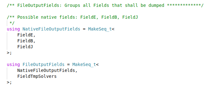
I don't know what is this feedback. I have this in the fieldOurput.param
cbontoiu
on 11 Mar 2020
Thank you for your corrections about the time step. I modified the grid.param file accordingly.
There is problem here though because using
constexpr float_64 DELTA_T_SI = 0.9999 / SPEED_OF_LIGHT_SI * sqrt( 1.0 / (1. / CELL_WIDTH_SI**2 + 1. / CELL_HEIGHT_SI**2 + 1/CELL_DEPTH_SI**2));
in my grid.param file give me this error
......grid.param(35): error #75: operand of "*" must be a pointer
so I had to insert the calculated value.
I also have a few questions:
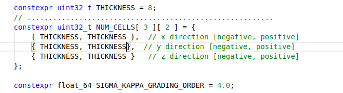
- What happens if during the laser-matter interactions particles enter the cells which bear the absorber/PML condition? Are they affected in any way?
- Are the absorber/PML layers meant to prevent laser/wave reflection back into the simulation domain?
- Should I initialize the laser (plane wave) with
initPlaneY = 0such that the absorber/PML layers in the left Y region are disabled? Should I initialize the laser inside the absorber/PML layer for example withinitPlaneY = 16for 32 absorber/PML cells. Should I do it just after this layer with ``initPlaneY = 33```? - Should there be a few void cells between the left Y absorber/PML layer and the matter, such that the laser progresses a number of cells in vacuum before hitting the target?
Thank you.
cbontoiu
on 11 Mar 2020
Hello @cbontoiu , CELL_WIDTH_SI**2 is notation in some programming languages, but not in C++. The simplest way is just to have (CELL_WIDTH_SI*CELL_WIDTH_SI) instead, and similarly for other variables. The brackets might be necessary for priority of operations.
Regarding the absorber questions.
- In the current implementation particles in the absorber areas are not affected while they are still in the simulation volume for both exponential damping and PML. However, the particles leaving the simulation area through these boundaries are removed. We understand this might be suboptimal, but do not plan to change it immediately.
- Yes, so they simulate free space where ideally outgoing waves never return back to the simulation area. Exponential damping just decays any waves inside, while PML only absorbs orthogonal to the boundary part, but the motivation is the same.
initPlaneY = 0is a special case, if this is enabled we will not do absorption at that boundary during the laser duration (even when you set this boundary as non-periodic) and enable it later. So in this case absorber and laser are never operating together. In case you setinitPlaneY > 0it has to be outside of the absorber width on that boundary, and this should be checked at compile time (please report if this check also does not work as intended!). So for 32 cells of any of the two absorbers (tho it is way too large for PML in my opinion, 16 should be very good already) please setinitPlaneY = 33.- I think this might indeed be useful with the current implementation in mind, also taking into account the Yee cells with staggered components.
sbastrakov
on 11 Mar 2020
@cbontoiu There is definitely something fishy with the ionization pattern you see.
I have seen a standing wave pattern before in an overdense setup where the laser that propagated in the medium ionized it and then the rest of the laser would feel the increase in electron density which caused it to blueshift. The waves started to catch up with one another and cause an oscillating field spike that always fluctuated around the BSI threshold of the next charge state.
Here is an image of that setup to illustrate this effect.
So I'd also be really interested in the absolute electric field from that simulation.
I would also recommend choosing either the normal BSI or the BSIStarkShifted which seems to overlap better with the regions where the tunneling models level out.
I quickly calculated that in that first GIF that you show you also only seem to resolve your laser period with 4 sample points which are very few. In the setup folder you sent that resolution is increased, however.
For this extremely short wavelength (Keldysh parameter for C1, and C2 for the maximum intensity of this setup are 6.93 and 10.21, respectively - and if >> 1: multi-photon regime) the target is fully transparent. The electric field could really help and show what's happening there.
Another thing that seems concerning: if you look at E_kin from the e_energy_all.dat you can see that in the end of the simulation all of your electrons have a combined energy in the MegaJoule range. I assume you do not have a laser that delivers MJ of energy to the target. ^^ So there might be really strong numerical heating happening. In a 2D simulation you would expect your particles to receive orders of magnitude less energy than the full laser pulse carries because you're just simulating a slice.
You could plot fields_energy.dat against e_energy_all.dat to see where/when things really diverge.
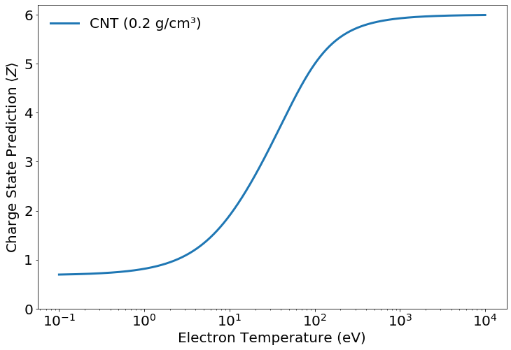
I checked the ThomasFermi model for its prediction at the CNT density and you can see that everything gets ionized drastically between 1 and 100 eV of electron temperature.
I assume your single-particle electron energies are unphysically high there.
Did the suggestions of the others already change the results?
 n01r
on 11 Mar 2020
n01r
on 11 Mar 2020
Thank you all for your help,
The model I present here is solved on a very rough grid and the laser enters at the 33rd cell directly in the tube. I will correct this.
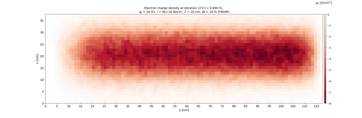
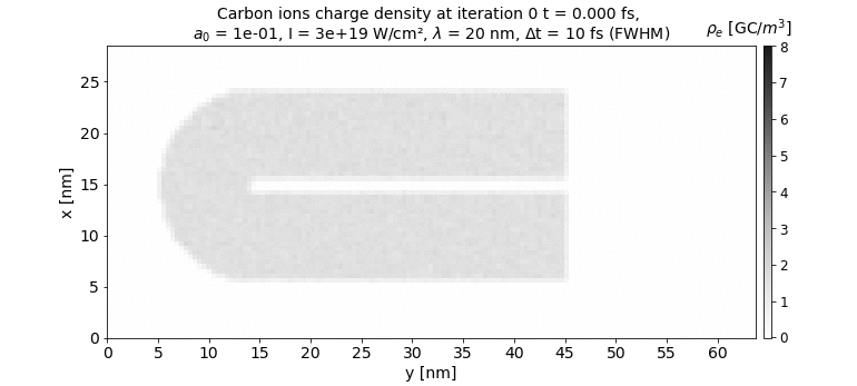
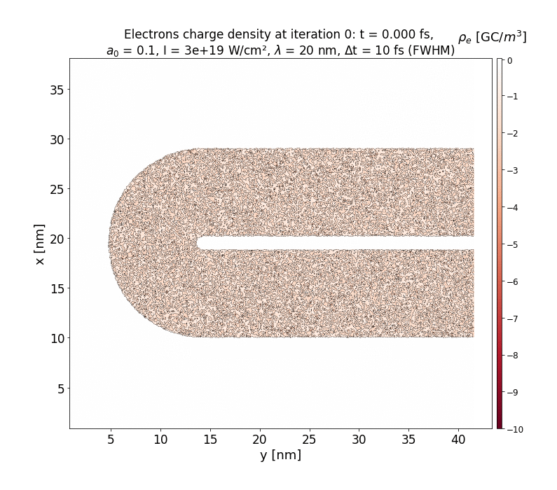
I removed the ionization by collision and the beam is not lost anymore. With only BSIEffectiveZ< Electrons > and ADKLinPol< Electrons > the electrons and carbon ions charge is as shown below. I used the classical Yee solver here with the new time step as advised above.
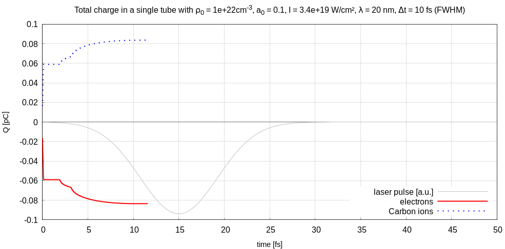
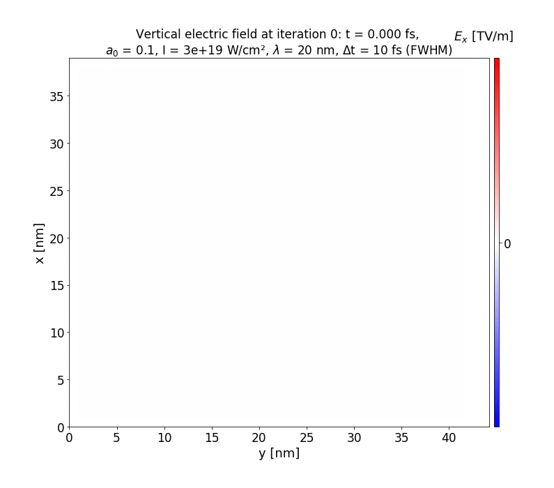
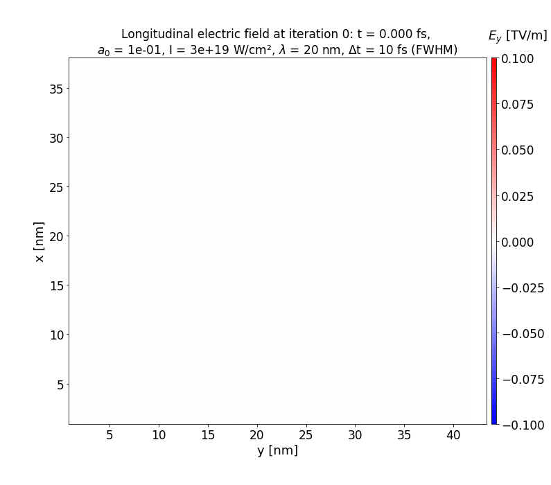
The electric field is strongest in the vertical X component as it comes from the laser. I did increase the a0 potential to 0.1, a value which I have never used before, being afraid of destroying the target completely. As you can see in the last 25 snapshots (just before the pulse maximum) there are really standing waves
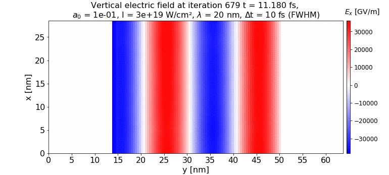
and this explains why charge gathers in the minima regions. The density is 1e28 1/m3 as calculated analytically for carbon nano tubes. I limited the right y-axis span of my tube, to stay out of the absorber.
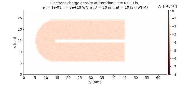
Carbon ions stay still
and here are other relevant plots.
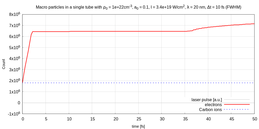
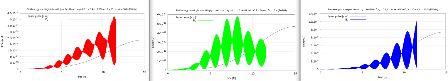
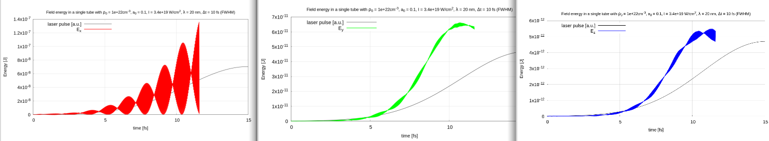
but I don't know how to interpret them yet.
and the interrupted output file with typical macro particle weighting: 0.151947
output.txt
I don't know what could I do with the h5 files which apper in two dedicated folders because I use in my cfg file:
TBG_e_countPerSuper="--e_macroParticlesPerSuperCell.period 19"
TBG_C_countPerSuper="--C_macroParticlesPerSuperCell.period 19"
Is is something that I do wrong? Should I trust the result? Please note that 20 nm that I use for the laser is actually much shorter than the plasma wavelength, 334 nm in this case.
Thank you!
Cristian
P.S. An observation for the cfg file:
although I use something like
TBG_sumEnergy="--fields_energy.period 73 --e_energy.period 73 --e_energy.filter all"
the energy will be listed for all iterations not every 73rd iteration. I am not sure which way is intended but it seems not to be consistent with the usual period syntax.
cbontoiu
on 11 Mar 2020
Did you find out what the problem was, @cbontoiu?
n01r
on 15 Mar 2020
Did you find out what the problem was, @cbontoiu?
Yes, I found the solution. I will upload some movies with my results. for the moment I think only YeePML solver gives the travelling wave expected solution, or at least this is how I got rid of the standing wave pattern for the Ex laser field.
cbontoiu
on 16 Mar 2020
Hello,
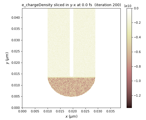
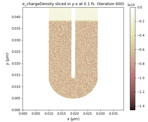
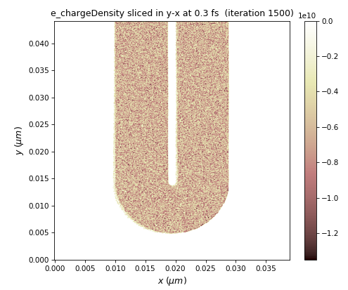
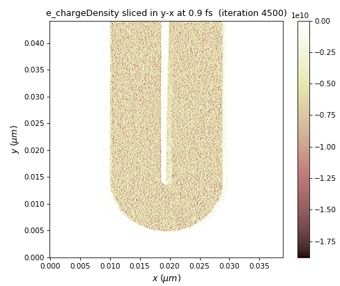
Here are some results using the YeePML solver. There is some problem with the right y-edge, because it makes my tube collapse leftwards, but maybe there is nothing else to do other than extending the structure and neglecting the right side results. The plots below are shown excluding 8 cells (absorber) from left-Y side and 24 cells (3 times the absorber) from the right Y-side:
- the electron charge density:
- the laser transverse electric field Ex
- the longitudinal (generated due to the tube) electric field Ey
Here is the complete input folder
one-tube-thick-parallel-LX.zip
cbontoiu
on 17 Mar 2020
Yes, your box simply seems too short.
Do you have access to more computing resources to make it longer?
However, it seems wide enough. What would you say @sbastrakov? D'you see anything abnormal/ any boundary effects transversally?
n01r
on 18 Mar 2020
Thanks for reporting @cbontoiu . This looks suspicious to me as well. Looking now.
@n01r as far as I see in the 1.cfg in the attached archive, that simulation only used absorbers along Y (which by itself is fine and should not cause any issues with PML).
sbastrakov
on 18 Mar 2020
Ah, right, there were periodic boundary conditions transversally.
Still, I'm a little concerned by the standing wave of the other solvers. ^^;
Would be good if we could pinpoint why that happened.
n01r
on 18 Mar 2020
Thanks for reporting @cbontoiu . This looks suspicious to me as well. Looking now.
@n01r as far as I see in the
1.cfgin the attached archive, that simulation only used absorbers along Y (which by itself is fine and should not cause any issues with PML).
If you refer to tha latest archive, I wonder how can you know about the absorbers from the 1.cfg file? There is only the periodicity there as TBG_periodic="--periodic 1 0 1"? Does it mean that enabling the periodicity disables the aborber layers on both sides? It make sense so. Also I recall that enabling periodicity at the X edges for example makes the particles which excced the the lower x-limit of the simulation domain, appear moving downwards across the upper x-limit. Is this as it should be with periodic conditions?
cbontoiu
on 18 Mar 2020
Yes @cbontoiu , absorbers (both PML and exponential damping) only work for axes with periodic set to 0. Since the periodic property is for both the min and max border, it is set for each of 3 axes, and not 6 borders separately. So in your 1.cfg the absorber was activated for the min and max Y borders. It is still possible to effectively disable one of those by setting the corresponding size to 0 if needed.
sbastrakov
on 18 Mar 2020
Yes, your box simply seems too short.
Do you have access to more computing resources to make it longer?
However, it seems wide enough. What would you say @sbastrakov? D'you see anything abnormal/ any boundary effects transversally?
Thank you for looking to my results. This simulation took 38 hours on my computer. For the moment I don't know how to run the code on a cluster, but I just got acceess to one at Liverpool University. I am in the process of learning.
If you have a chance you could run the files in the last zip folder using other solvers and check for the standing waves. The zip-folder attached in this thread, one-tube-thick.zip should result in such a situation, but I don't rember all differences between the two simulation cases.
It would be very useful if you could spot the differences between the two zip folders and clarify. Is there a bug with the solvers or, is there an unlucky condition that I set in the first case?
cbontoiu
on 18 Mar 2020
For spotting the differences please use diff -r [directory1] [directory2]. Earlier in that thread there were also commands to get the list of files that are different, not the differences themselves.
sbastrakov
on 18 Mar 2020
Hello @cbontoiu , I tried to reproduce by running the setup in one-tube-thick-parallel-LX.zip. The one-tube-thick.zip as attached does not match the CFL condition - now the PML solver also checks it. There are also other differences between the two, as shown by diff -r (described in the previous message).
I am confused by values of dt and t in the gifs you attached for the ...parallel-LX version. Here the actual dt = 0.0002 fs. This does not match 10 fs in your pictures, but also even t in the .gifs is not equal to iteration multiplied by 10 fs. However, I assume this is just a visualization inconsistency due to changes in the setup, and not different simulation parameters. If the parameters were indeed different, please attach the up-to-date version.
I ran that setup for 5000 iterations. Just FYI, on a Tesla V100 GPU these iterations took 33 minutes. I did not observe the deformations in electron change density, attaching a couple of pictures. Sorry for not making a gif, I had some difficulty with doing it, but I think even from these pictures some differences are seen from your .gifs. I also did not see visible laser reflections from the absorber. Your original 1.cfg uses a much larger number of time steps: 144896, so I only simulated the very start. Are the iterations numbers in your .gifs also for the very start of the run? So basically something does not match, I am not sure what.
sbastrakov
on 19 Mar 2020
Hello, thanks for looking into this. The simulation resulted in more than a thousand files, as I am sampling four times per laser period. A .gif with all of them would be in the order of 5-7 MB and impossible to upload on github. Even the Jupyter kernel dies if overloaded. What I do instead is to write out an image every 50 files or so and then upload here
https://ezgif.com/maker
to create the gif. This is why you see less snapshots in the uploaded gifs. However, even in your last picture I see the electrons fluctuating; with 5000 iterations you are just in the beginning of the laser pulse and the electric field is still small.
I will keep you updated on this problem of the standing waves as soon as I notice it again, but so far I am happy with the latest model and I managed to work with longer tubes at lower meshing. The next step I have to do is to include the ionization by collision and maybe decrease a0 not to pulverize the target below the minimum weight.
Cheers,
Cristian
cbontoiu
on 19 Mar 2020
I don't know what is this feedback. I have this in the
fieldOurput.param
Sorry for the delayed answer: The feedback I meant was the current deposition. But it was my mistake - you chose the default current deposition scheme by not setting (due to not having a species.param). I was confused with the current interpolation method, which was set to None in your fieldSolver.param - but this is all fine.
PrometheusPi
on 24 Mar 2020
@cbontoiu FYI we just discovered a bug in the dev version regarding the exponential absorber. It was there since February 20 and will be fixed today with #3218. Perhaps this can explain the standing waves in all solvers but YeePML, since that was the only non-affected solver+absorber combination.
sbastrakov
on 26 Mar 2020
Related issues
 saipavankalyan
·
3Comments
cbontoiu
·
3Comments
saipavankalyan
·
3Comments
cbontoiu
·
3Comments
 psychocoderHPC
·
4Comments
cbontoiu
·
3Comments
psychocoderHPC
·
4Comments
cbontoiu
·
3Comments
 hightower8083
·
4Comments
hightower8083
·
4Comments
Most helpful comment
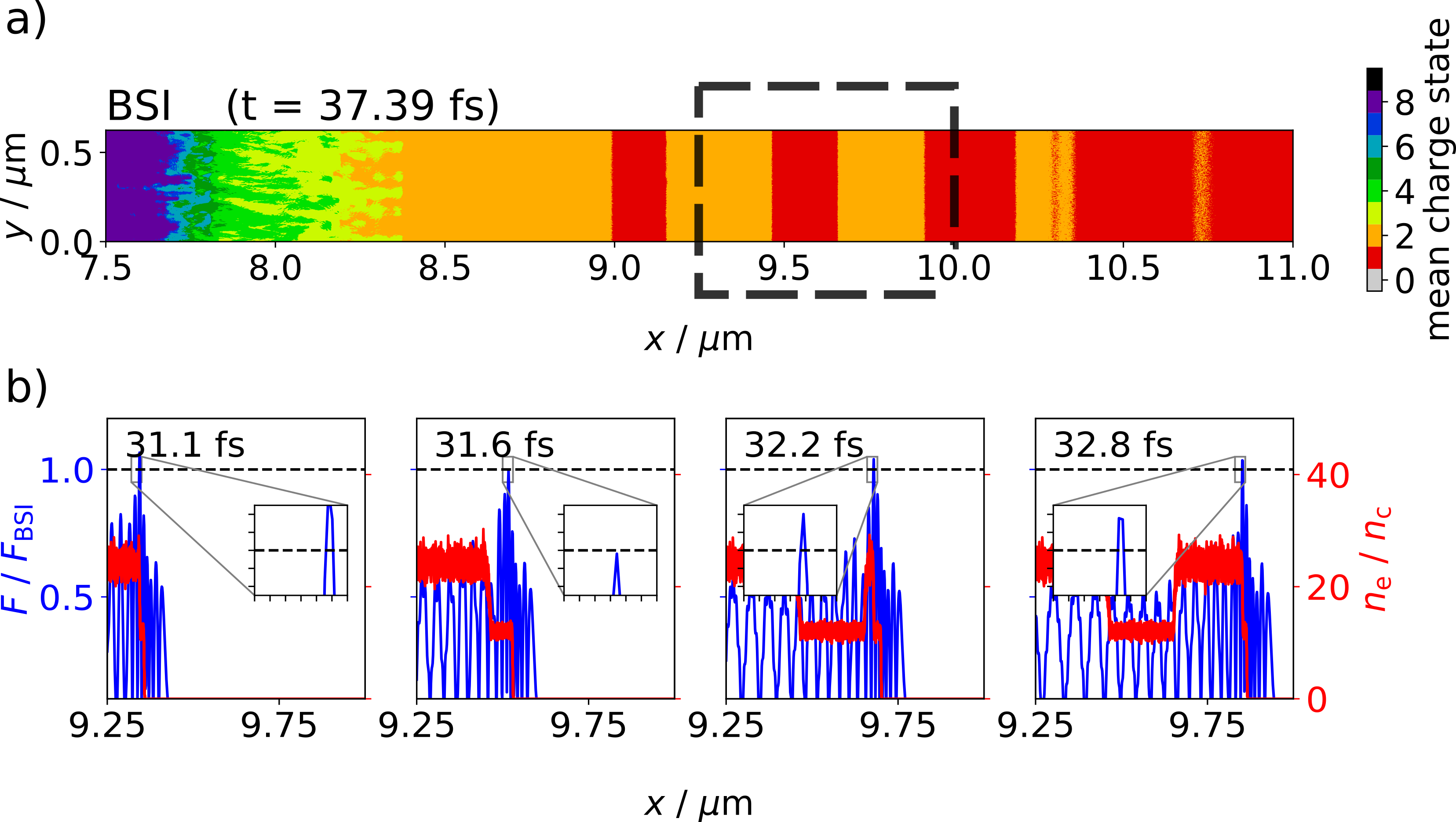
@cbontoiu There is definitely something fishy with the ionization pattern you see.
I have seen a standing wave pattern before in an overdense setup where the laser that propagated in the medium ionized it and then the rest of the laser would feel the increase in electron density which caused it to blueshift. The waves started to catch up with one another and cause an oscillating field spike that always fluctuated around the BSI threshold of the next charge state.
Here is an image of that setup to illustrate this effect.
So I'd also be really interested in the absolute electric field from that simulation.
I would also recommend choosing either the normal
BSIor theBSIStarkShiftedwhich seems to overlap better with the regions where the tunneling models level out.I quickly calculated that in that first GIF that you show you also only seem to resolve your laser period with 4 sample points which are very few. In the setup folder you sent that resolution is increased, however.
For this extremely short wavelength (Keldysh parameter for C1, and C2 for the maximum intensity of this setup are 6.93 and 10.21, respectively - and if >> 1: multi-photon regime) the target is fully transparent. The electric field could really help and show what's happening there.
Another thing that seems concerning: if you look at E_kin from the
e_energy_all.datyou can see that in the end of the simulation all of your electrons have a combined energy in the MegaJoule range. I assume you do not have a laser that delivers MJ of energy to the target. ^^ So there might be really strong numerical heating happening. In a 2D simulation you would expect your particles to receive orders of magnitude less energy than the full laser pulse carries because you're just simulating a slice.You could plot
fields_energy.datagainste_energy_all.datto see where/when things really diverge.I checked the

ThomasFermimodel for its prediction at the CNT density and you can see that everything gets ionized drastically between 1 and 100 eV of electron temperature.I assume your single-particle electron energies are unphysically high there.
Did the suggestions of the others already change the results?