Picongpu: laser-carbon interaction

[cbontoiu]

I am a bit confused on what happens in my model attached as params files and 1.cfg file. I insert a laser beam as defined in the official thin-foil example. One one hand I try to learn how to move the laser beam along the X-axis such that it strikes the charge density ribbons not at the base but at an arbitrary point. The first question is how to do it, because I cannot find the answer in the manual. The second question is why the applied tilt is not visible? On a TBG_gridSize="640 4352" grid with the aspect ratio ~1/7 the applied 45 deg tilt should be visible.

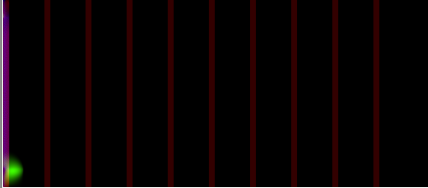
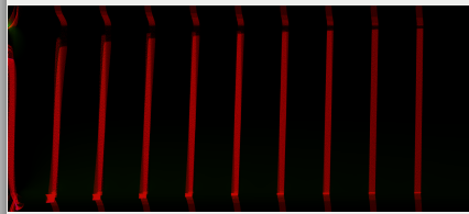
On the other hand just looking at the pictures for the electrons I can notice slight green color region at the top-left corner of the image attached. This means field_E.x() as defined in the png.param, but where does it come since the laser pulse is gone? Is it a numerical error? Another question is why do the tubes appear as fractured? There was no periodicity applied in the 1.cfg file. I thing the gap and if the electrons density and the top-left electric field are related.

Any suggestion is highly appreciated.
Thanks

param.zip
1.cfg.txt

[sbastrakov]

Hello @cbontoiu

Your laser profile seem to be parametrized. What value of PARAM_LASERPROFILE did you use? Was it the PlaneWave as defined on top of the file, did you define PARAM_LASERPROFILE at compile time? Also, what time step is the attached pngs captured at?

[cbontoiu]

Hi Sergei,

Thanks for replying.
It was the same as in the thin foil example

ifndef PARAM_LASERPROFILE

define PARAM_LASERPROFILE PlaneWave

....
using Selected = PARAM_LASERPROFILE< PMACC_JOIN( PARAM_LASERPROFILE, Param )>;

and the snapshots are produced as

TBG_epngYX="--e_png.period 100 --e_png.axis yx --e_png.slicePoint 0.5 --e_png.folder pngElectronsYX"

and I show the second one (top) e_png_yx_0.5_000100.png and the last one (bottom) e_png_yx_0.5_006000.png I assume the unit is what I use in grid.param, that is constexpr float_64 DELTA_T_SI = CELL_WIDTH_SI / ( 1.415 * SPEED_OF_LIGHT_SI );

[sbastrakov]

Thanks for clarifications. Without running + tweaking a simulation (for me) it's hard to tell exactly. Just from the top of my head, it might be that 45 degree tilt works not the way you expected. How the tilt works is that the pulse still propagates along y but just the front is not orthogobal to the y axis (and keeps that way). Is it your intention?

[psychocoderHPC]

There are a few small issues in the setup.

• Your target begins in the initial plain of the laser. You should keep vacum at the beginning.
  e.g. change your density functor to

HDINLINE float_X
operator()( const floatD_64& position_SI, const float3_64& cellSize_SI )
{
    if(position_SI.y()/cellSize_SI.y() < 240)
      return 0.;
...

I would suggest to change the laser too and set static constexpr uint32_t initPlaneY = 80u;. Than the absorber on the left (in the image, y direction in the simulation) will be enabled.

You are using the PlainWave laser, this laser has an infinite size in the transversal direction (x in the simulation) therefore you should set in the cfg file periodic boundaries for the x direction to avoid artifacts on the borders. TBG_periodic="--periodic 1 0"

This means field_E.x() as defined in the png.param, but where does it come since the laser pulse is gone?

In this file you map the green color to channel 2 namespace preChannel2Col = colorScales::green; the definition of the channel 2 is at the end of the file

        DINLINE float_X preChannel2(const float3_X& field_B, const float3_X& field_E, const float3_X& field_J)
        {
            return field_E.x();
        }

So you plotted the x component of the electric field. The color is adjusted per image automatically #define EM_FIELD_SCALE_CHANNEL2 -1

Please keep in mind that the png's are only a preview of the simulation. YOu should always use adios or hdf5 to analyze the simulation.

The reason why you do not see any laser in the simulation could come from the very high sampling of the laser wave. In output you find PIConGPUVerbose PHYSICS(1) | y-cells per wavelength: 200000. This mean you need to simulate 200k iterations to see one wavelength.