Lightgbm: Alpha for quantile regression doesn't seem to work

[elaser]

Hi there!
I've been working with @ClimbsRocks on using auto_ml as a wrapper on top of lightgbm for a lot of our use cases at work. We're super excited that lightgbm supports quantile regression. I saw earlier in #1036 that it looks like alpha issue was resolved, but when I pass in different alphas, I'm not seeing different results.

On my end, I wrote some functions to check if there were any difference between passing in alpha=.86 and alpha=.95 and I keep on getting results that were ~ 58th percentile as opposed to 86th or 95th on my validation and test sets.

@ClimbsRocks wrote something to test this:

%matplotlib inline
import numpy as np
import matplotlib.pyplot as plt


## ADDED
import lightgbm as lgb
## END ADDED


from sklearn.ensemble import GradientBoostingRegressor

np.random.seed(1)


def f(x):
    """The function to predict."""
    return x * np.sin(x)

#----------------------------------------------------------------------
#  First the noiseless case
X = np.atleast_2d(np.random.uniform(0, 10.0, size=10000)).T
X = X.astype(np.float32)

# Observations
y = f(X).ravel()

dy = 1.5 + 1.0 * np.random.random(y.shape)
noise = np.random.normal(0, dy)
y += noise
y = y.astype(np.float32)

# Mesh the input space for evaluations of the real function, the prediction and
# its MSE
xx = np.atleast_2d(np.linspace(0, 10, 100000)).T
xx = xx.astype(np.float32)

alpha = 0.95

# clf = GradientBoostingRegressor(loss='quantile', alpha=alpha,
#                                 n_estimators=250, max_depth=3,
#                                 learning_rate=.1, min_samples_leaf=9,
#                                 min_samples_split=9)

# clf.fit(X, y)


## ADDED
clf = lgb.LGBMRegressor(objective='quantile',
                        alpha=alpha,
                        num_leaves=31,
                        learning_rate=0.05,
                        n_estimators=100)
clf.fit(X, y,
        eval_set=[(X, y)],
        eval_metric='quantile',
        early_stopping_rounds=5)
## END ADDED


# Make the prediction on the meshed x-axis
y_upper = clf.predict(xx)

# clf.set_params(alpha=1.0 - alpha)
# clf.fit(X, y)


## ADDED
clf.set_params(alpha=1.0 - alpha)
clf.fit(X, y,
        eval_set=[(X, y)],
        eval_metric='quantile',
        early_stopping_rounds=5)
## END ADDED


# Make the prediction on the meshed x-axis
y_lower = clf.predict(xx)

# clf.set_params(loss='ls')
# clf.fit(X, y)


## ADDED
clf.set_params(objective='regression', eval_metric='l2')
clf.fit(X, y,
        eval_set=[(X, y)],
        eval_metric='l2',
        early_stopping_rounds=5)
## END ADDED


# Make the prediction on the meshed x-axis
y_pred = clf.predict(xx)

# Plot the function, the prediction and the 90% confidence interval based on
# the MSE
fig = plt.figure()
plt.plot(xx, f(xx), 'g:', label=u'$f(x) = x\,\sin(x)$')
plt.plot(X, y, 'b.', markersize=10, label=u'Observations')
plt.plot(xx, y_pred, 'r-', label=u'Prediction')
plt.plot(xx, y_upper, 'k-')
plt.plot(xx, y_lower, 'k-')
plt.fill(np.concatenate([xx, xx[::-1]]),
         np.concatenate([y_upper, y_lower[::-1]]),
         alpha=.5, fc='b', ec='None', label='90% prediction interval')
plt.xlabel('$x$')
plt.ylabel('$f(x)$')
plt.ylim(-10, 20)
plt.legend(loc='upper left')
plt.show()

and was seeing something like:

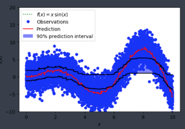
Is alpha hardcoded in somewhere or is this user error on my end?

[guolinke]

@wxchan @StrikerRUS can you help to debug this? I think the alpha parameter is not passed right in python package

[wxchan]

@guolinke I add a log to print out config.alpha here https://github.com/Microsoft/LightGBM/blob/8ebef94cfe0627aef6def578fb0e6a2e082dbf1e/src/metric/regression_metric.hpp#L143, I think alpha is successfully set.

[guolinke]

can you try following:

1. reduce the number of points, e.g. 1000
2. more iterations with larger learning rate

[elaser]

i played with the parameters, and here's one of the outputs

My parameters are

{'num_leaves': 8, 'learning_rate': 0.3, 'lambda_l2': 0.001, 'n_estimators': 1000, 'num_iteration': 10, 'histogram_pool_size': 16384}

and I'm seeing results like:

('Number of quantile estimate >= actual_offset: ', 369870)
('Number of quantile estimate < actual_offset: ', 267464)

It doesn't seem to be much different from the result of running non-quantile regression

[guolinke]

did you use the latest master code?
And early stopping may be the reason.

[elaser]

early stopping? like not enough estimators? I installed latest from master and still seeing similar results.

[guolinke]

@elaser
just try it with 0.99 and 0.9 . the result is normal:

import numpy as np
import matplotlib.pyplot as plt


## ADDED
import lightgbm as lgb
## END ADDED


from sklearn.ensemble import GradientBoostingRegressor

np.random.seed(1)


def f(x):
    """The function to predict."""
    return x * np.sin(x)

#----------------------------------------------------------------------
#  First the noiseless case
X = np.atleast_2d(np.random.uniform(0, 10.0, size=10000)).T
X = X.astype(np.float32)

# Observations
y = f(X).ravel()

dy = 1.5 + 1.0 * np.random.random(y.shape)
noise = np.random.normal(0, dy)
y += noise
y = y.astype(np.float32)

# Mesh the input space for evaluations of the real function, the prediction and
# its MSE
xx = np.atleast_2d(np.linspace(0, 10, 10000)).T
xx = xx.astype(np.float32)

alpha = 0.99

# clf = GradientBoostingRegressor(loss='quantile', alpha=alpha,
#                                 n_estimators=250, max_depth=3,
#                                 learning_rate=.1, min_samples_leaf=9,
#                                 min_samples_split=9)

# clf.fit(X, y)


## ADDED
clf = lgb.LGBMRegressor(objective='quantile',
                        alpha=alpha,
                        num_leaves=31,
                        learning_rate=0.1,
                        n_estimators=1000)
clf.fit(X, y,
        eval_set=[(X, y)],
        eval_metric='quantile')
## END ADDED


# Make the prediction on the meshed x-axis
y_upper = clf.predict(xx)

# clf.set_params(alpha=1.0 - alpha)
# clf.fit(X, y)


## ADDED
clf.set_params(alpha=1.0 - alpha)
clf.fit(X, y,
        eval_set=[(X, y)],
        eval_metric='quantile')
## END ADDED


# Make the prediction on the meshed x-axis
y_lower = clf.predict(xx)

# clf.set_params(loss='ls')
# clf.fit(X, y)


## ADDED

alpha=0.9
clf.set_params(alpha=alpha)
clf.fit(X, y,
        eval_set=[(X, y)],
        eval_metric='quantile')
## END ADDED


# Make the prediction on the meshed x-axis
y_upper_90 = clf.predict(xx)

# clf.set_params(alpha=1.0 - alpha)
# clf.fit(X, y)


## ADDED
clf.set_params(alpha=1.0 - alpha)
clf.fit(X, y,
        eval_set=[(X, y)],
        eval_metric='quantile')
## END ADDED


# Make the prediction on the meshed x-axis
y_lower_10 = clf.predict(xx)


## ADDED
clf.set_params(objective='regression', eval_metric='l2')
clf.fit(X, y,
        eval_set=[(X, y)],
        eval_metric='l2',
        early_stopping_rounds=5)
## END ADDED


# Make the prediction on the meshed x-axis
y_pred = clf.predict(xx)

# Plot the function, the prediction and the 90% confidence interval based on
# the MSE
fig = plt.figure()
plt.plot(xx, f(xx), 'g:', label=u'$f(x) = x\,\sin(x)$')
plt.plot(X, y, 'b.', markersize=10, label=u'Observations')
plt.plot(xx, y_pred, 'r-', label=u'Prediction')
plt.plot(xx, y_upper, 'k-')
plt.plot(xx, y_lower, 'k-')


plt.plot(xx, y_upper_90, 'y-')
plt.plot(xx, y_lower_10, 'y-')


plt.xlabel('$x$')
plt.ylabel('$f(x)$')
plt.ylim(-10, 20)
plt.legend(loc='upper left')
plt.show()

[guolinke]

for the quantile, you need to run with much more iteration. it is hard to convergence.
you also can set reg_sqrt=True to speed up the convergence.

import numpy as np
import matplotlib.pyplot as plt


## ADDED
import lightgbm as lgb
## END ADDED


from sklearn.ensemble import GradientBoostingRegressor

np.random.seed(1)


def f(x):
    """The function to predict."""
    return x * np.sin(x)

#----------------------------------------------------------------------
#  First the noiseless case
X = np.atleast_2d(np.random.uniform(0, 10.0, size=10000)).T
X = X.astype(np.float32)

# Observations
y = f(X).ravel()

dy = 1.5 + 1.0 * np.random.random(y.shape)
noise = np.random.normal(0, dy)
y += noise
y = y.astype(np.float32)

# Mesh the input space for evaluations of the real function, the prediction and
# its MSE
xx = np.atleast_2d(np.linspace(0, 10, 10000)).T
xx = xx.astype(np.float32)

alpha = 0.99

# clf = GradientBoostingRegressor(loss='quantile', alpha=alpha,
#                                 n_estimators=250, max_depth=3,
#                                 learning_rate=.1, min_samples_leaf=9,
#                                 min_samples_split=9)

# clf.fit(X, y)


## ADDED
clf = lgb.LGBMRegressor(objective='quantile',
                        alpha=alpha,
                        num_leaves=31,
                        learning_rate=0.1,
                        n_estimators=100,
                        reg_sqrt=True)
clf.fit(X, y,
        eval_set=[(X, y)],
        eval_metric='quantile')
## END ADDED


# Make the prediction on the meshed x-axis
y_upper = clf.predict(xx)

# clf.set_params(alpha=1.0 - alpha)
# clf.fit(X, y)


## ADDED
clf.set_params(alpha=1.0 - alpha)
clf.fit(X, y,
        eval_set=[(X, y)],
        eval_metric='quantile')
## END ADDED


# Make the prediction on the meshed x-axis
y_lower = clf.predict(xx)

# clf.set_params(loss='ls')
# clf.fit(X, y)


## ADDED

alpha=0.9
clf.set_params(alpha=alpha)
clf.fit(X, y,
        eval_set=[(X, y)],
        eval_metric='quantile')
## END ADDED


# Make the prediction on the meshed x-axis
y_upper_90 = clf.predict(xx)

# clf.set_params(alpha=1.0 - alpha)
# clf.fit(X, y)


## ADDED
clf.set_params(alpha=1.0 - alpha)
clf.fit(X, y,
        eval_set=[(X, y)],
        eval_metric='quantile')
## END ADDED


# Make the prediction on the meshed x-axis
y_lower_10 = clf.predict(xx)


## ADDED
clf.set_params(objective='regression', eval_metric='l2')
clf.fit(X, y,
        eval_set=[(X, y)],
        eval_metric='l2',
        early_stopping_rounds=5)
## END ADDED


# Make the prediction on the meshed x-axis
y_pred = clf.predict(xx)

# Plot the function, the prediction and the 90% confidence interval based on
# the MSE
fig = plt.figure()
plt.plot(xx, f(xx), 'g:', label=u'$f(x) = x\,\sin(x)$')
plt.plot(X, y, 'b.', markersize=10, label=u'Observations')
plt.plot(xx, y_pred, 'r-', label=u'Prediction')
plt.plot(xx, y_upper, 'k-')
plt.plot(xx, y_lower, 'k-')


plt.plot(xx, y_upper_90, 'y-')
plt.plot(xx, y_lower_10, 'y-')


plt.xlabel('$x$')
plt.ylabel('$f(x)$')
plt.ylim(-10, 20)
plt.legend(loc='upper left')
plt.show()

[elaser]

thanks @guolinke -- i bumped up the learning rate and added reg_sqrt=True and that made all the difference!

[joseortiz3]

Why is quantiles being set in so many places? objective, metric, eval_metric......In the sklearn version, you set it once and done.

[Laurae2]

@joseortiz3 because you might want to observe something else than quantile loss when performing quantile regression (such as mse, mae, etc. or a self-defined business metric). For a quantile task, in most cases you will watch the MSE metric and not the quantile metric.

[joseortiz3]

Thanks @Laurae2 .

I'm having problems with the quantiles functionality converging far too slowly to be useful. It's a little hard to explain what is going on, but I will try. It might come down to the data I'm using too (stock volumes have a funny distribution) - but then again maybe not.

In my application (prediction of stock trading volumes), it doesn't seem like this quantile functionality is a good substitute for the quantile functionality in sklearn at this point. Sklearn is able to converge to an accurate estimate of the quantile using the following default parameters:

{'alpha': 0.9, 'criterion': 'friedman_mse', 'init': None, 'learning_rate': 0.1, 'loss': 'quantile', 'max_depth': 3, 'max_features': None, 'max_leaf_nodes': None, 'min_impurity_decrease': 0.0, 'min_impurity_split': None, 'min_samples_leaf': 1, 'min_samples_split': 2, 'min_weight_fraction_leaf': 0.0, 'n_estimators': 100, 'presort': 'auto', 'random_state': None, 'subsample': 1.0, 'verbose': 0, 'warm_start': False}

The default parameters in LightGBM are much faster - in my problem training takes 7s, compared to 125s for sklearn, but do converge to very poor estimates of the quantile - the estimate ends up being nearly identical to the non-quantile regression, even for very large or small alphas.

{'boosting_type': 'gbdt', 'colsample_bytree': 1.0, 'learning_rate': 0.1, 'max_depth': -1, 'min_child_samples': 20, 'min_child_weight': 0.001, 'min_split_gain': 0.0, 'n_estimators': 100, 'n_jobs': -1, 'num_leaves': 31, 'objective': 'quantile', 'random_state': None, 'reg_alpha': 0.0, 'reg_lambda': 0.0, 'silent': True, 'subsample': 1.0, 'subsample_for_bin': 200000, 'subsample_freq': 1}

Also, for my data, the predictions end up showing severe under-fitting, with almost every prediction being nearly the same.

If I instead bump the number of iteratations, n_estimators, to over 4000, I can get decent estimates comparable to sklearn, but it takes far longer single-thread than sklearn does single-thread. Also quantiles_l2 behaves much, much better than quantiles does, but not good enough.

I also tried matching some parameters between LightGBM and SKLearn, such as setting max_depth to 3, but nothing worked out. I also tried messing around with the available tree parameters, such as num_leaves and reg_sqrt as suggested. Nothing worked.

I wonder if there is something wrong with the quantiles code? Or perhaps the method of growing trees LightGBM uses (leaf-wise, not level-wise) is not suitable for use with your standard quantile loss function [that I know nothing about]? (based only on the observation that sklearn is able to get good quantile estimates with far fewer iterations)

In total, can someone explain why obtaining an quantile estimate is so difficult, what can be done to more-quickly obtain a quantiles estimate, and what might currently be wrong with the quantiles code, if anything?

--

Also the "solution" to the problem posted here has some flaws - for instance the "inside-curve" portions have very poor quantile estimates. It's not clear if the quantile estimate is failing when y~0 or from the convexity of the function its simulating around x in [7,9] etc

[guolinke]

@joseortiz3
The main difference is the leaf_output. Sklearn use the according percentile value as output, while LightGBM uses gradients (much smaller values) directly.
As a result, you can use larger learning_rate, e.g. 0.3 or 0.4.
You also can set reg_sqrt to True to speed up the convergence.

quantile_l2 uses the second order gradients, so it will be faster. However, it is more easily over-fitting.

[joseortiz3]

It still seems that no matter the setting or label transformation, sklearn converges with much less iterations (by an order of magnitude) to an accurate quantile estimate than lightGBM does. (Although I'm not sure if it's fair to compare sklearn and lightGBM iterations)

It's interesting that reg_sqrt helps, since f(x) = sqrt(x) is just one example of a one-to-one mapping that squishes fat-tailed distributions closer to the origin. This reminded me of the importance of making sure your prediction target is nicely distributed - in my case I think most of the slow convergence comes from the extremely skewed distribution of stock volumes. It did much better after I applied reg_sqrt, but even better once I applied log(1 + label / constant). Yet, still not as robust as sklearn it seems even when sklearn is trained on the original, un-transformed targets. The sklearn code doesn't seem to be applying any sort of transformations to the targets, and it apparently does not need to.

I did see that they use a quantile target calculated from scipy.stats.scoreatpercentile, which is a median-like function, not a mean-like function; it just sorts the targets and interpolates to find the target value at the percentile. Perhaps the definition of a quantile between sklearn and lightgbm is different? I.e. sklearn's is like a median, but lightgbm's is like a mean? Then maybe both are performing correctly, just at two different tasks. Is this possible?

--

Edit: I tried using sklearn.preprocessing to transform the targets to either a uniform or normal distribution. The sklearn quantiles still did an amazing job, while the lightGBM did an ok job but was _poorly-calibrated_ - setting a quantile of 0.6 for instance results in an effective quantile of 0.3, etc, for this skewed dataset that sklearn has no problem with.

It's this alpha-_calibration_ problem that I've decided for the purposes of my work is not functioning correctly. All alpha settings result in a much smaller effective alpha.

I think maybe an issue should be raised or development should be taken to better-calibrate the alpha setting, because right now it's really not calibrated convincingly.

[guolinke]

@joseortiz3
Yeah, the reason the calculation of leaf-output.

LightGBM's output is based on objective function (quantile loss), whose gradients are fixed values:
https://github.com/Microsoft/LightGBM/blob/master/src/objective/regression_objective.hpp#L395-L401 .
And the leaf-output is sum_grad / sum_hess. As a result, its outputs have no relation with the label magnitude. So using reg_sqrt can help convergence, since it reduces range of labels.

For the sklearn, though its gradient is also based on quantile loss. However,
its output is based on label(y) directly. So it will be much faster. : https://github.com/scikit-learn/scikit-learn/blob/c9e6d4d3a42b966b5f00725a0fce52c5517c933e/sklearn/ensemble/gradient_boosting.py#L434-L442

quantile_l2 uses similar strategy, it changes the quantile loss to L2 form, as a result, the gradients will be related to the magnitude of labels. : https://github.com/Microsoft/LightGBM/blob/master/src/objective/regression_objective.hpp#L443-L449