I generated this map with googleVis::gvisGeoMap

I can generate something very similar with leaflet
library(rgdal)
library(leaflet)
library(dplyr)

# From https://www.census.gov/geo/maps-data/data/cbf/cbf_state.html
states <- readOGR(dsn = "./cb_2014_us_state_20m.shp",
                  layer = "cb_2014_us_state_20m", verbose = FALSE)

my_counts <- data.table(
  State = c(
    "CA", "TX", "IL", "FL", "NY", "OH",
    "NJ", "GA", "MI", "PA", "MA", "CO", "AZ", "NC", "VA", "WA", "IN",
    "MD", "MN", "WI", "MO", "TN", "IA", "KY", "LA", "SC", "CT", "AL",
    "KS", "OR", "OK", "AR", "NV", "UT", "NE", "ID", "MS", "DC", "NM",
    "NH", "ME", "AK", "RI", "MT", "HI", "WV", "SD", "ND", "DE", "VT",
    "WY", "PR", "GU", "VI", "MP", "AS", "na", "MH", "FM", "PW"
  ),
  count = c(
    1590533L, 1016328L, 754535L, 742603L, 714205L,
    538719L, 477278L, 452064L, 437162L, 428616L, 420332L, 391084L,
    380853L, 354601L, 342533L, 335505L, 294670L, 286026L, 273427L,
    246172L, 238968L, 236037L, 235030L, 209514L, 199013L, 191707L,
    185521L, 179931L, 163477L, 159862L, 142610L, 136006L, 120111L,
    117338L, 112671L, 106176L, 102564L, 100168L, 97496L, 69881L,
    69508L, 68684L, 65631L, 62109L, 61123L, 57300L, 57254L, 56091L,
    51696L, 33944L, 32136L, 4822L, 598L, 468L, 49L, 19L, 17L,
    11L, 2L, 1L
  )
)


my_counts <- my_counts %>%  filter(State %in% states$STUSPS) %>% mutate(State=factor(State))

df1 <- merge(states, my_counts, by.x="STUSPS", by.y="State", all.x=TRUE, suffixes = c(".x",".y"))

#make map
map <- leaflet(df1)

pal <- colorNumeric(
  palette = "YlGnBu",
  domain = df1$count
)
map %>%
  addPolygons(stroke = FALSE, smoothFactor = 0.2, fillOpacity = 1,
              color = ~pal(count)
  ) %>%
  addLegend("topright", pal = pal, values = ~count,
            title = "Count",
            opacity = 1
  ) %>% setView(lng = -100.0167, lat = 50.8833, zoom = 3)
Is it possible to move and resize Alaska and Hawaii so the leaflet map looks like the gvisGeoMap map?
 ignacio82
All 11 comments
Try this (requires maptools I think):
https://rstudio-pubs-static.s3.amazonaws.com/94122_462a1d171e4944f0a99c1f91fd5071d5.html#move-alaska-scaled-down-and-hawaii
 jcheng5
on 26 Aug 2015
jcheng5
on 26 Aug 2015
@jcheng5 I'm able to follow that tutorial to generate a ggplot2 map. This is the code that I'm using:
remove.territories = function(.df) {
subset(.df,
.df$id != "AS" &
.df$id != "MP" &
.df$id != "GU" &
.df$id != "PR" &
.df$id != "VI"
)
}
x = c("ggplot2", "rgdal", "maptools", "mapproj", "rgeos")
lapply(x, library, character.only = TRUE)
plain_theme = theme(axis.text=element_blank()) +
theme(panel.background = element_blank(),
panel.grid = element_blank(),
axis.ticks = element_blank())
no_ylab = ylab("")
no_xlab = xlab("")
# From https://www.census.gov/geo/maps-data/data/cbf/cbf_state.html
us <- readOGR(dsn = "./cb_2014_us_state_5m.shp",
layer = "cb_2014_us_state_5m", verbose = FALSE)
# convert it to Albers equal area
us_aea <- spTransform(us, CRS("+proj=laea +lat_0=45 +lon_0=-100 +x_0=0 +y_0=0 +a=6370997 +b=6370997 +units=m +no_defs"))
us_aea@data$id <- rownames(us_aea@data)
# extract, then rotate, shrink & move alaska (and reset projection)
# need to use state IDs via # https://www.census.gov/geo/reference/ansi_statetables.html
alaska <- us_aea[us_aea$STATEFP=="02",]
alaska <- elide(alaska, rotate=-50)
alaska <- elide(alaska, scale=max(apply(bbox(alaska), 1, diff)) / 2.3)
alaska <- elide(alaska, shift=c(-2100000, -2500000))
proj4string(alaska) <- proj4string(us_aea)
# extract, then rotate & shift hawaii
hawaii <- us_aea[us_aea$STATEFP=="15",]
hawaii <- elide(hawaii, rotate=-35)
hawaii <- elide(hawaii, shift=c(5400000, -1400000))
proj4string(hawaii) <- proj4string(us_aea)
# remove old states and put new ones back in; note the different order
# we're also removing puerto rico in this example but you can move it
# between texas and florida via similar methods to the ones we just used
us_aea <- us_aea[!us_aea$STATEFP %in% c("02", "15", "72"),]
us_aea <- rbind(us_aea, alaska, hawaii)
us50 <- fortify(us_aea, region="STUSPS")
us50 = remove.territories(us50)
#plot
p = ggplot(data=us50) +
geom_map(map=us50, aes(x=long, y=lat, map_id=id, group=group), ,fill="white", color="dark grey", size=0.15) +
no_ylab +
no_xlab +
plain_theme
p
The problem is that I end up with a data frame us50 that is not compatible with leaflet.
library(leaflet)
leaflet(us50) %>%
addPolygons(stroke = FALSE, fillOpacity = 0.5, smoothFactor = 0.5)
Error in polygonData.default(data) :
Don't know how to get path data from object of class data.frame
Is us50 not a SpatialPolygonsDataFrame? How about us_aea?
On Tue, Sep 1, 2015 at 6:14 PM ignacio82 [email protected] wrote:
@jcheng5 https://github.com/jcheng5 I'm able to follow that tutorial to
generate a ggplot2 map. This is the code that I'm using:remove.territories = function(.df) {
subset(.df,
.df$id != "AS" &
.df$id != "MP" &
.df$id != "GU" &
.df$id != "PR" &
.df$id != "VI"
)
}x = c("ggplot2", "rgdal", "maptools", "mapproj", "rgeos")
lapply(x, library, character.only = TRUE)
plain_theme = theme(axis.text=element_blank()) +
theme(panel.background = element_blank(),
panel.grid = element_blank(),
axis.ticks = element_blank())no_ylab = ylab("")
no_xlab = xlab("")From https://www.census.gov/geo/maps-data/data/cbf/cbf_state.html
us <- readOGR(dsn = "./cb_2014_us_state_5m.shp",
layer = "cb_2014_us_state_5m", verbose = FALSE)convert it to Albers equal area
us_aea <- spTransform(us, CRS("+proj=laea +lat_0=45 +lon_0=-100 +x_0=0 +y_0=0 +a=6370997 +b=6370997 +units=m +no_defs"))
us_aea@data$id <- rownames(us_aea@data)extract, then rotate, shrink & move alaska (and reset projection)
need to use state IDs via # https://www.census.gov/geo/reference/ansi_statetables.html
alaska <- us_aea[us_aea$STATEFP=="02",]
alaska <- elide(alaska, rotate=-50)
alaska <- elide(alaska, scale=max(apply(bbox(alaska), 1, diff)) / 2.3)
alaska <- elide(alaska, shift=c(-2100000, -2500000))
proj4string(alaska) <- proj4string(us_aea)extract, then rotate & shift hawaii
hawaii <- us_aea[us_aea$STATEFP=="15",]
hawaii <- elide(hawaii, rotate=-35)
hawaii <- elide(hawaii, shift=c(5400000, -1400000))
proj4string(hawaii) <- proj4string(us_aea)remove old states and put new ones back in; note the different order
we're also removing puerto rico in this example but you can move it
between texas and florida via similar methods to the ones we just used
us_aea <- us_aea[!us_aea$STATEFP %in% c("02", "15", "72"),]
us_aea <- rbind(us_aea, alaska, hawaii)
us50 <- fortify(us_aea, region="STUSPS")
us50 = remove.territories(us50)plot
p = ggplot(data=us50) +
geom_map(map=us50, aes(x=long, y=lat, map_id=id, group=group), ,fill="white", color="dark grey", size=0.15) +
no_ylab +
no_xlab +
plain_theme
pThe problem is that I end up with a data frame us50 that is not
compatible with leaflet.library(leaflet)
leaflet(us50) %>%
addPolygons(stroke = FALSE, fillOpacity = 0.5, smoothFactor = 0.5)
Error in polygonData.default(data) :
Don't know how to get path data from object of class data.frame—
Reply to this email directly or view it on GitHub
https://github.com/rstudio/leaflet/issues/172#issuecomment-136908315.
jcheng5
on 2 Sep 2015
@jcheng5
us50is not aSpatialPolygonsDataFrame, it is a normal data frameus_aeais aSpatialPolygonsDataFrame, but I cannot plot it with leaflet. When i try I just get an empty gray area.
Thanks!
ignacio82
on 2 Sep 2015
fortify seems to be a ggplot2/ggmap specific thing, let's not do that.
I think the reason us_aea is not working is because it's been projected to Albers. I didn't notice that when I sent you the link. Sorry, I think you'll need to find a different version of this code, that uses unprojected coordinates.
Honestly, I think you might get better help from r-sig-geo at this point.
jcheng5
on 2 Sep 2015
@jcheng5 is correct, this is more of a generic issue on spatial objects (hence r-sig-geo is the right place to take up the question).
you need to transform you data back again. following should get you going:
us_aea2 <- spTransform(us_aea, proj4string(us))
map <- leaflet(us_aea2)
pal <- colorNumeric(
palette = "YlGnBu",
domain = us_aea2$ALAND)
map %>%
addPolygons(stroke = FALSE, smoothFactor = 0.2, fillOpacity = 1,
color = ~pal(ALAND))
regards,
einar
 einarhjorleifsson
on 2 Sep 2015
einarhjorleifsson
on 2 Sep 2015
Thanks a lot!
ignacio82
on 2 Sep 2015
Did you have any luck? Its been two years but google still doesn't produce anything that answers this question.
 jzadra
on 25 Oct 2017
jzadra
on 25 Oct 2017
I guess not :(
jzadra
on 16 Aug 2018
You can use the albersusa package to have Alaska and Hawaii placed more conveniently:
# devtools::install_github("hrbrmstr/albersusa")
library(albersusa)
library(leaflet)

# map without background map
leaflet(options = leafletOptions(crs = leafletCRS(crsClass = "L.CRS.Simple"),
                                 minZoom = -100)) %>%
  addPolygons(data = usa_sf("lcc"))

# with background map (which is of course non-sense)
leaflet() %>%
  addTiles() %>%
  addPolygons(data = usa_sf("longlat"))
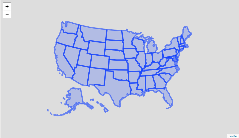

 tim-salabim
on 16 Aug 2018
tim-salabim
on 16 Aug 2018
Albersusa is awesome, just noting that usa_sf() is a dataset, so you can replace the geometries of your own dataset as shown here:
library(albersusa) # see the github for state and counties moved.
library(sf) # for st_drop_geometry()
my_spatial_data <- readRDS("myspatialdata.rds")
move_akhi <- usa_sf()
move_akhi$State <- move_akhi$iso_3166_2 # state abbrevation column, AK, AL ...
geometry <- move_akhi[,"State"] # subsetting class sf always retains geometry
my_spatial_data <- merge(x = geometry, y = st_drop_geometry(my_spatial_data),
             by = "State", all.x = TRUE)
 CR-Mercado
on 13 Mar 2019
CR-Mercado
on 13 Mar 2019
Related issues
 gdmcdonald
·
4Comments
gdmcdonald
·
4Comments
 ideamotor
·
7Comments
ideamotor
·
7Comments
 loerasg
·
6Comments
loerasg
·
6Comments
 BastienFR
·
5Comments
BastienFR
·
5Comments
 yyz1989
·
7Comments
yyz1989
·
7Comments
Most helpful comment
You can use the albersusa package to have Alaska and Hawaii placed more conveniently: