Turing.jl: addlogprob not working when sampling from prior

[drbenvincent]

I'm experimenting with imposing an order constraint in the Turing model like this

if θ1 > θ2
    Turing.@addlogprob! Inf
end

And I'm coming across some unexpected behaviour. The order constraint seems to work when sampling from the posterior, but not when sampling from the prior.

using Turing, StatsPlots

s1 = 250
s2 = 500
n1 = 500
n2 = 1000

@model function model(s1, s2, n1, n2)
    θ1 ~ Uniform(0, 1)
    θ2 ~ Uniform(0, 1)
    # order constraint
    if θ1 > θ2
        Turing.@addlogprob! Inf
    end
    δ = θ1 - θ2
    s1 ~ Binomial(n1, θ1)
    s2 ~ Binomial(n2, θ2)
    return δ
end

# sample from prior
prior_chain = sample(model(s1, s2, n1, n2), Prior(), 2000)
δprior = generated_quantities(model(s1, s2, n1, n2), prior_chain)

# sample from posterior
posterior_chain = sample(model(s1, s2, n1, n2), NUTS(), 10_000)
δ = generated_quantities(model(s1, s2, n1, n2), posterior_chain)

plot(layout=(2, 2), size=(600, 600))
scatter!(prior_chain[:θ1], prior_chain[:θ2], subplot=1, title="samples from prior", legend=false, xlabel="θ1", ylabel="θ2")
histogram!(δprior, subplot=3, xlabel="δprior", legend=false)
scatter!(posterior_chain[:θ1], posterior_chain[:θ2], subplot=2, title="samples from posterior", legend=false, xlabel="θ1", ylabel="θ2")
histogram!(δ, subplot=4, xlabel="δ", legend=false)

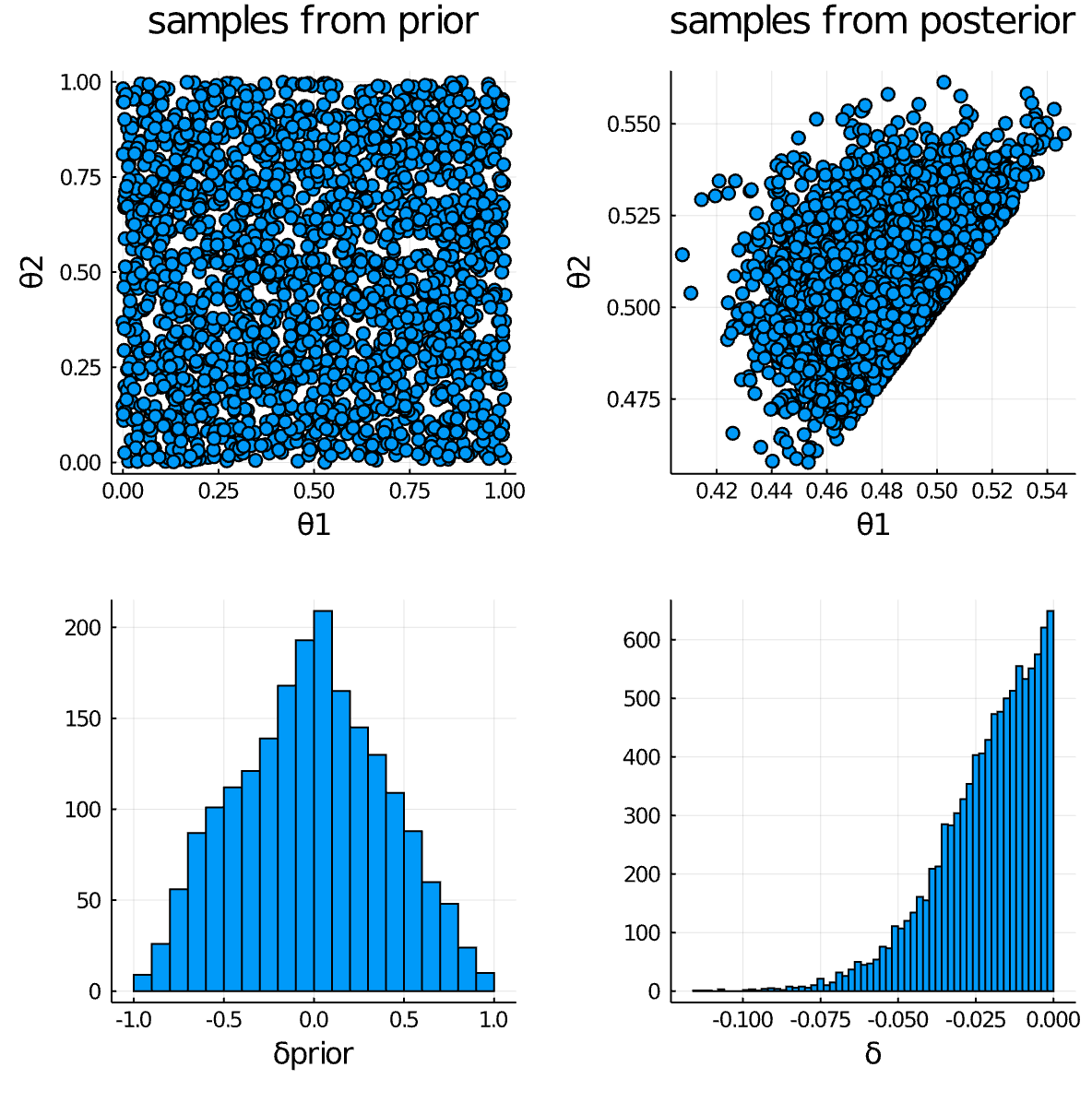
There should be no samples from the prior (top left) where θ1 > θ2 (ie the lower right triangle of that plot should be empty). Correspondingly there should not be any positive values of δprior (lower left). The use of Turing.@addlogprob! Inf does seem to be working when sampling from the posterior, but not the prior.

I'm assuming this is a bug?

[luiarthur]

I don't know enough about the internals to answer your question.

But are you trying to impose that θ2 > θ1? In that case, I think you would want

if θ1 > θ2
    Turing.@addlogprob! -Inf  # should have a negative sign
end

This way, when θ1 > θ2, you multiply the unnormalized joint posterior density by 0 instead of infinity.

Still, I don't know if this actually works in Turing.

But I would think that the Turing parser doesn't know whether the constraint belongs to the prior or the likelihood (someone correct me if I'm wrong).

[luiarthur]

Another way to write the model, if you want 0 < theta1 < theta2 < 1, would be:

theta1 ~ Uniform(0, 1)
theta2 ~ Uniform(theta1, 1)

[drbenvincent]

Thanks for inputs @luiarthur

theta1 ~ Uniform(0, 1)
theta2 ~ Uniform(theta1, 1)

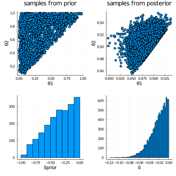
So this is a good idea. It half does the job. This is taken from an example from a book that I'm converting into Turing.jl models. It highlights that using that method will produce bias when calculating a Bayes factor over δ = θ1 - θ2. For example, doing what you suggest, gives this distribution of samples on the left. But using the order constraint (when working correctly, see below) gives you a more correct set of prior samples (right).

See how you get a higher density in one part of the space, which will give a bias for the prior over δ. You can see it in this plot... it's a rubbish plot, but you get the idea. You have an inflated prior density for δ near zero. This may normally not be a problem, but it _is_ a problem if you are using that prior to work out a Bayes Factor.

I can get it working using an approach where you explicitly add in variables for the prior which are unattached to the data.

@model function model2(s1, s2, n1, n2)
    θ1 ~ Uniform(0, 1)
    θ2 ~ Uniform(0, 1)
    θ1prior ~ Uniform(0, 1)
    θ2prior ~ Uniform(0, 1)
    # order constraint
    if (θ1 > θ2) | (θ1prior > θ2prior)
        Turing.@addlogprob! -Inf
    end
    δ = θ1 - θ2
    δ_prior = θ1prior - θ2prior
    s1 ~ Binomial(n1, θ1)
    s2 ~ Binomial(n2, θ2)
    return (δ, δ_prior)
end

So essentially I can solve my problem. But I felt that the order constraint not working when sampling from the prior in the way suggested (eg prior_chain = sample(model(s1, s2, n1, n2), Prior(), 2000)) could potentially be a bug.

But yes... I don't know if Turing.@addlogprob! is supposed to just affect the likelihood alone? Either way, it seemed like a deviation from expected behaviour.

[luiarthur]

You're absolutely right; these are different priors.

One thing you might do instead is define a custom multivariate Distribution for theta1 and theta2 so you get the intended prior.

I think in this case, all you would need to implement are Distributions.rand and Distributions.logpdf.

[drbenvincent]

At this point I'm still a bit new to Turing (and Julia), so I will see if I can make progress on translating other models first. But at some point, trying my hand at a custom distribution sounds fun.

[luiarthur]

Fair enough. Here's the reference to creating a custom Distribution:
https://juliastats.org/Distributions.jl/latest/extends/

[luiarthur]

So, a complete solution would be more involved, as a Bijector needs to be implemented for this constrained prior for gradient-based samplers. But this works with Metropolis-Hastings:

# Import libraries.
using Turing
using Distributions
using Random
import StatsFuns: logtwo  # just a constant for log(2)

# Define a new Distribution called OrderedBivariateUniform
struct OrderedBivariateUniform{T<:Real} <: ContinuousMultivariateDistribution end

# Some helper methods. See:
# https://juliastats.org/Distributions.jl/latest/extends/#Create-a-Distribution
Base.length(::OrderedBivariateUniform{<:Real}) = 2
Base.eltype(::Type{<:OrderedBivariateUniform{T}}) where {T} = T

# This is called by `rand`.
function Distributions._rand!(rng::AbstractRNG, d::OrderedBivariateUniform{<:Real},
                              x::AbstractArray)
  x .= 0.5
  while x[1] >= x[2]
    x[1] = rand(rng)
    x[2] = rand(rng)
  end
  return x
end

# This is called by `logpdf`
function Distributions._logpdf(d::OrderedBivariateUniform{<:Real}, x::AbstractArray)
  return 0 <= x[1] < x[2] <= 1 ? logtwo : -Inf
end

# TODO: Implement a Bijector ...

### Example: ###

# Define model.
@model function demo(s1, s2, n1, n2)
  u ~ OrderedBivariateUniform{Float64}()
  s1 ~ Binomial(n1, u[1])
  s2 ~ Binomial(n2, u[2])
  delta = u[1] - u[2]
  return delta
end

# Instantiate model.
m = demo(250, 500, 500, 1000)

# Get prior samples
prior_samples = sample(m, Prior(), 2000)

# Get posterior samples
posterior_samples = sample(m, MH(), 2000, discard_initial=100, thinning=100)

# Get deltas.
delta_prior_samples = generated_quantities(m, prior_samples)
delta_posterior_samples = generated_quantities(m, posterior_samples)

[drbenvincent]

This is excellent @luiarthur. I will take a proper look in the morning.

I’d still be interested in hearing from someone if the addlogprob! is supposed to affect the prior, or if there is an alternative to target the prior. From a practitioner perspective, being able to define a model with an order constraint as in the original post would be really attractive in its simplicity.

EDIT: having thought about it, the solution of a custom prior is much better. The addlogprob! is more of a kludge imperative hack in this case. The custom prior is a much more elegant way of describing the model you want

[luiarthur]

@xukai92 Any thoughts on this? Particularly, regarding sampling from the prior in the original post.

[luiarthur]

Apparently, this is a very interesting problem. So I came up with another solution:

@model function demo(s1, s2, n1, n2)
  u ~ filldist(Uniform(), 2)
  u1 = minimum(u)
  u2 = maximum(u)
  s1 ~ Binomial(n1, u1)
  s2 ~ Binomial(n2, u2)
  delta = u1 - u2
  return delta
end

This way, we don't create a new Distribution, and gradient-based algorithms (e.g. HMC, NUTS) and sampling from the prior would work. In general, I think you can do this to impose ordering in the way you want:

@model function demo(ss, ns)  # ss and ns are vectors, and assuming length(ss) == length(ns)
  u_unsorted ~ filldist(Uniform(), length(ss))
  u = sort(u_unsorted)
  ss .~ Binomial.(ns, u)
end

I'll think about this more.

[torfjelde]

Just to add to what's going on here.

Sampling from the prior will simply call rand on the prior distributions. As a result, even if the actual logprob is -Inf they can still be sampled if it's allowed by the rand implementation for the prior. As a result, you have two options:

1. Implement your own prior distribution which correctly won't sample value with -Inf logprob.
2. Filter the chain obtained using Prior to only contain samples with finite logprob.

(1) is exactly what @luiarthur nicely demonstrated above. For (2), you can do:

indices = findall(isfinite, vec(prior_chain[:lp]));

# `resetrange` is to make make the indices of the samples to be `1:length(chain)`
prior_chain = resetrange(prior_chain[indices, :, :])
δprior = generated_quantities(model(s1, s2, n1, n2), prior_chain)

The annoying bit here is that the number of samples won't be what you want since you've now dropped a large number of the original 2000 samples.

But, if you really want to, you can make use of the new iterator interface for AbstractMCMC as follows:

# Setup
m = model(s1, s2, n1, n2)
num_samples = 2_000

# Internally `Prior` uses this for sampling, though note that `Prior` 
# is a `Turing.InferenceAlgorithm` and `DynamicPPL.SampleFromPrior` is a `DynamicPPL.AbstractSampler`.
# See https://turing.ml/dev/docs/for-developers/how_turing_implements_abstractmcmc for more on this, if you're really interested.
spl = DynamicPPL.SampleFromPrior()

# Construct an iterator for the model `m` with the sampler `spl`
prior_iterator = AbstractMCMC.steps(m, spl)

# Get the initial sample
state, _ = iterate(prior_iterator)

# Use initial sample to construct a container for the samples
samples = AbstractMCMC.samples(state, m, spl)

# Iterate until we have the desired number of samples
while length(samples) < num_samples
    state, _ = iterate(prior_iterator, state)

    # Only accept those with non-zero probability or, equivalently, `-Inf` log-probability
    if isfinite(DynamicPPL.getlogp(state))
        AbstractMCMC.save!!(samples, state, length(samples) + 1, m, spl)
    end
end

# Convert the `samples` container into a `MCMCChains.Chains` instance
prior_chain = AbstractMCMC.bundle_samples(samples, m, spl, state, MCMCChains.Chains)

and then you can just call generated_quantities as before to obtain the desired result! :tada:

[drbenvincent]

@model function demo(s1, s2, n1, n2)
  u ~ filldist(Uniform(), 2)
  u1 = minimum(u)
  u2 = maximum(u)
  s1 ~ Binomial(n1, u1)
  s2 ~ Binomial(n2, u2)
  delta = u1 - u2
  return delta
end

This is great and very creative. This is the solution that I will go with. It effectively implements the prior that is intended, but without the verbosity of formally creating a new distribution.

[drbenvincent]

Thanks for these answers - very informative and thorough. I'm still getting used to the fact that you can just use arbitrary julia code in your models (within limits?). Hopefully I'll get an opportunity to use this kind of approach to solve related problems that come up.

[xukai92]

An alternative is simply to sample from the prior by HMC. Here is the modefied code:

using Turing, StatsPlots

s1 = 250
s2 = 500
n1 = 500
n2 = 1000

@model function model(s1, s2, n1, n2; prior=false)
    θ1 ~ Uniform(0, 1)
    θ2 ~ Uniform(0, 1)
    # order constraint
    if θ1 > θ2
        Turing.@addlogprob! Inf
    end
    if !prior
        δ = θ1 - θ2
        s1 ~ Binomial(n1, θ1)
        s2 ~ Binomial(n2, θ2)
        return δ
    end
end

# sample from prior
prior_chain = sample(model(s1, s2, n1, n2; prior=true), NUTS(), 2000)
δprior = generated_quantities(model(s1, s2, n1, n2), prior_chain)

# sample from posterior
posterior_chain = sample(model(s1, s2, n1, n2), NUTS(), 10_000)
δ = generated_quantities(model(s1, s2, n1, n2), posterior_chain)

and the result

All I did is adding a keyword argument to optionally create a "prior model".

[luiarthur]

Thanks @torfjelde and @xukai92 for the additional thoughts! Also, I think in the example above, the intention was

Turing.@addlogprob! -Inf

[luiarthur]

@drbenvincent do you think we can close this issue now?

[xukai92]

Thanks @torfjelde and @xukai92 for the additional thoughts! Also, I think in the example above, the intention was

Turing.@addlogprob! -Inf

Makes sense. I merely copy-pasted the code from the original post. I guess in this case Inf is treated as numerical error and got rejected.

[drbenvincent]

@drbenvincent do you think we can close this issue now?

Thanks all for the very thorough responses