Statsmodels: ETS(M, A, M) gives exploding forecasts

[mustafaaydn]

Describe the bug

Trying to forecast a monthly series from M4 data with statsmodels.tsa.exponential_smoothing.ets.ETSModel using "MAM" formulation, I get forecast values that explode compared to series' values.

Code Sample, a copy-pastable example if possible

here is the series:

import numpy as np
series = np.array([ 696.1,  691.7,  690.5,  694. ,  696.9,  701.4,  701.2,  704.8,
        703.5,  702.9,  700.9,  699. ,  700.5,  698.8,  699.6,  699.1,
        702.8,  705.9,  712.9,  715.1,  715.9,  711.7,  713.3,  713.3,
        715. ,  712.6,  714.9,  719.4,  725.3,  729.2,  733.3,  736.1,
        738.7,  739.1,  739.7,  742.7,  747.2,  750.8,  752.1,  752.6,
        757.1,  761.5,  766. ,  768.8,  769.5,  772.5,  775.6,  779.5,
        781.6,  782.6,  783.2,  784. ,  785.5,  787.6,  791.4,  795.7,
        799. ,  801. ,  801.8,  803.8,  807. ,  809.7,  811. ,  814.9,
        818.5,  822.6,  823. ,  826.1,  829.3,  831.4,  833.6,  833.3,
        835.4,  835.4,  837.8,  843.7,  850.3,  853.8,  856.1,  857.5,
        862.6,  865.2,  869.5,  870.9,  874. ,  876. ,  882. ,  890.3,
        898.6,  904.9,  907.6,  909.9,  912.8,  919.5,  925.5,  929.5,
        932.9,  936.4,  943.4,  949.8,  959.1,  966.6,  973.2,  976.2,
        980.1,  985.9,  991.2,  997.6, 1000. , 1008. , 1011.8, 1025. ,
       1033.8, 1045.8, 1048.1, 1050.9, 1050.8, 1055.6, 1060.4, 1063.5,
       1066.3, 1069. , 1072.4, 1080.8, 1087.4, 1097.7, 1102.4, 1107.1,
       1110.9, 1112.4, 1111.7, 1110.1, 1111.8, 1116.7, 1120.2, 1123.9,
       1130.1, 1137.5, 1143.1, 1146.8, 1147.6, 1148.6, 1149.1, 1149.1,
       1151.2, 1152.3, 1158.4, 1160.6, 1168.8, 1173.5, 1177.9, 1181.7,
       1185.3, 1184. , 1184.5, 1183.1, 1186.7, 1186.5, 1190.6, 1201. ,
       1208.8, 1214.9, 1222.3, 1228.6, 1233.7, 1232.7, 1232.7, 1235.3,
       1238.4, 1242.1, 1247. , 1259.2, 1271.2, 1285.3, 1290.3, 1295.1,
       1294.9, 1296.3, 1298.3, 1302.1, 1305.9, 1306.1, 1306.2, 1315.1,
       1327.2, 1340.1, 1349. , 1352.7, 1351. , 1347.3, 1341.8, 1340.1,
       1334.5, 1333. , 1332.2, 1342.7, 1350.3, 1361.1, 1364.7, 1364.4,
       1355.5, 1338.6, 1313.4, 1296.1, 1277.6, 1259.8, 1244.6, 1236.2,
       1242.9, 1246.1, 1247.4, 1243.2, 1227.1, 1197.9, 1164.6, 1130. ,
       1094.4, 1066.5, 1050.7, 1054.2, 1059.8, 1076.2, 1100.9, 1112.7,
       1112.6, 1101.2, 1092.9, 1086.2, 1070.4, 1056.5, 1037.3, 1056.9,
       1078.6, 1097.2, 1100.2, 1089.5, 1063.9, 1033. , 1008. , 1000.6,
       1003.3, 1006.8, 1003.3, 1018.1, 1028. , 1043.2, 1045.5, 1020.4,
        959.9,  912.1,  889.2,  873. ,  854.4,  832.7,  825.4,  844.8,
        878.7,  917.5,  941.5,  958. ,  960.6,  956. ,  956.8,  959.5,
        969.8,  970.1,  982.5, 1020.1, 1055.1, 1091.5, 1115.4, 1134.7,
       1139.9, 1137.2])

from statsmodels.tsa.exponential_smoothing.ets import ETSModel

model = ETSModel(series, error="mul", trend="add", seasonal="mul", seasonal_periods=12)
results = model.fit()
forecasts = results.forecast(18)

forecasts, results.aic

This gives some warnings:

C:\Users\need-\Anaconda3\lib\site-packages\statsmodels\tsa\exponential_smoothing\ets.py:1135: RuntimeWarning:
invalid value encountered in log
  logL -= np.sum(np.log(yhat))

C:\Users\need-\Anaconda3\lib\site-packages\scipy\optimize\_numdiff.py:497: RuntimeWarning:
invalid value encountered in subtract
  df = fun(x) - f0

the forecasts:

array([  1383.98028445,   1996.90398876,   3298.65860508,   6621.25277208,
         25190.45397198, -23936.0908373 ,   9193.34409017,  12169.0775097 ,
         16174.92722858,   7414.38916173,   5031.07169576,   4305.69195626,
          4620.1267419 ,   5904.76719382,   8848.87505548,  16391.96804281,
         58292.39021889, -52285.31293353])

and the AIC: -inf.

Expected Output

Something similar to what happens in R with fpp3 package:

library("fpp3")

fit <- series %>%
    model(ETS(value ~ error("M") + trend("A") + season("M", period = 12)))

fit %>%
    forecast(h = 18) %>%
    pull(.mean)

 [1] 1133.705 1149.165 1168.920 1179.029 1202.016 1254.401 1307.556 1361.239
 [9] 1393.442 1409.058 1396.381 1375.134 1366.897 1381.559 1401.397 1409.698
[17] 1433.414 1492.076

Here is R's report on this model also:

Model: ETS(M,A,M) 
  Smoothing parameters:
    alpha = 0.5623894 
    beta  = 0.118081 
    gamma = 0.4354631 

  Initial states:
        l          b        s1       s2       s3       s4       s5        s6
 695.6708 -0.7641923 0.9878925 1.018886 1.002181 1.017573 1.001898 0.9858801
       s7       s8        s9       s10      s11      s12
 1.006929 1.009098 0.9836056 0.9803067 0.996579 1.009172

  sigma^2:  1e-04

     AIC     AICc      BIC 
2918.049 2920.440 2979.472 

I was actually trying AutoETS of sktime on some M4 series and this came up. (Since the AIC value is negative infinity, this model was selected; and R selects ETS(A,Ad,A) in automatic mode).

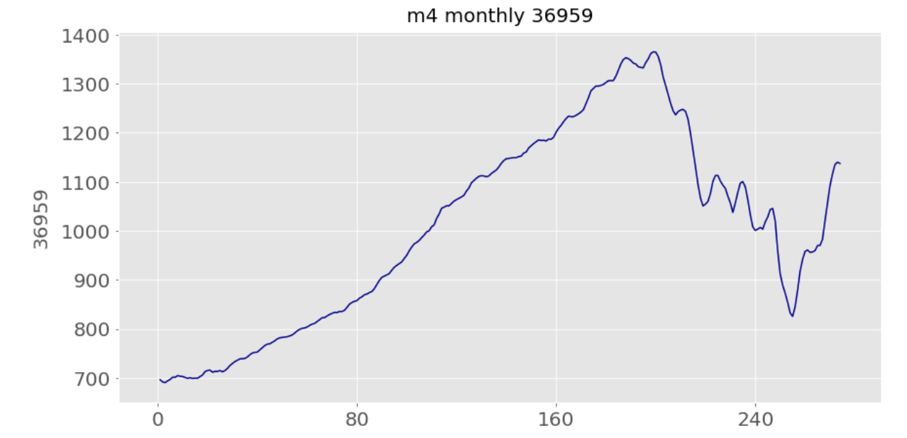
Lastly here are some plots from Python and R:

the series itself:

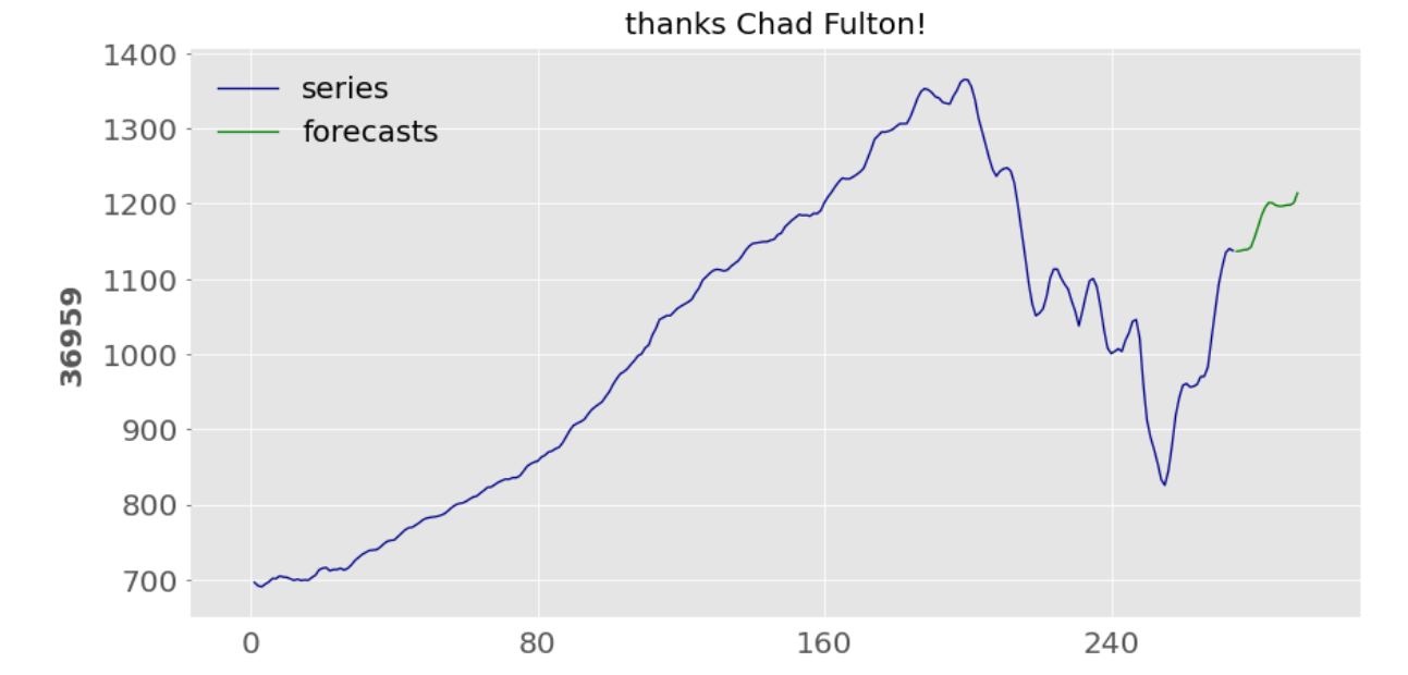
together with statsmodels' forecasts:

that of R:

Output of import statsmodels.api as sm; sm.show_versions()

INSTALLED VERSIONS

Python: 3.7.1.final.0

statsmodels

Installed: 0.12.2 (C:\Users\need-\Anaconda3\lib\site-packages\statsmodels)

Required Dependencies

cython: 0.29.21 (C:\Users\need-\Anaconda3\lib\site-packages\Cython)
numpy: 1.19.0 (C:\Users\need-\Anaconda3\lib\site-packages\numpy)
scipy: 1.5.0 (C:\Users\need-\Anaconda3\lib\site-packages\scipy)
pandas: 1.1.0 (C:\Users\need-\AppData\Roaming\Python\Python37\site-packages\pandas)
dateutil: 2.8.1 (C:\Users\need-\Anaconda3\lib\site-packages\dateutil)
patsy: 0.5.1 (C:\Users\need-\Anaconda3\lib\site-packages\patsy)

Optional Dependencies

matplotlib: 3.2.2 (C:\Users\need-\Anaconda3\lib\site-packages\matplotlib)
backend: module://ipykernel.pylab.backend_inline
cvxopt: Not installed
joblib: 0.15.1 (C:\Users\need-\Anaconda3\lib\site-packages\joblib)

Developer Tools

IPython: 7.15.0 (C:\Users\need-\AppData\Roaming\Python\Python37\site-packages\IPython)
jinja2: 2.11.2 (C:\Users\need-\Anaconda3\lib\site-packages\jinja2)
sphinx: 3.1.1 (C:\Users\need-\Anaconda3\lib\site-packages\sphinx)
pygments: 2.7.3 (C:\Users\need-\AppData\Roaming\Python\Python37\site-packages\pygments)
pytest: 5.4.3 (C:\Users\need-\Anaconda3\lib\site-packages\pytest)
virtualenv: Not installed

[ChadFulton]

Thanks very much for reporting this, I'll take a look at what we can do.

[ChadFulton]

This looks to me to be a practical example of the generic instability of models with an additive and multiplicative component along with the assumption of Gaussian errors. The multiplicative assumption is only valid with strictly positive data, but the data generating process will eventually produce a negative value. See for example Chapter 15 of Hyndman et al. (2008), especially the discussion at the end of 15.4.

In this case, the specific issue is that the one-step-ahead prediction eventually becomes less than zero, and then the log-likelihood is not well-defined. This is combined with (a) a shortcut used to assign an infinite value when this happens, and (b) a bug that assigned positive infinity rather than negative infinity.

However, I think that assigning negative infinity is not likely to produce good results with the numerical optimizer. Instead, I think that we could "clip" the predictions to be strictly positive but very small, so that taking the log yields an appropriately large negative value.

So currently we have (in the multiplicative errors case):

logL -= np.sum(np.log(yhat))  # problematic if yhat < 0
if np.isnan(logL):
    logL = np.inf  # even if we use this approach, should be -np.inf 

So one way to fix this would be:

yhat[yhat <= 0] = 1 / (1e-8 * (1 + np.abs(yhat[yhat < 0])))
logL -= np.sum(np.log(yhat))

This is ad hoc, but as I mentioned above, this entire class of models is in some sense ad hoc, as noted above.

[mustafaaydn]

Thanks for the enlightening explanation and the solution!

[ChadFulton]

Glad it worked! Thanks again for the report.