Statsmodels: How to generate SARIMAX out-of-sample simulations with last observations as initial condition

[andrmalm]

Hi! Let me try to explain what I want to achieve with my code:

First I want to fit a SARIMAX model "fitMdl" (with no seasonality in this case) using input data "fitData" (the observed time-series process) and "fitExog" (the only exogenous regressor). Then I want to initialize a new SARIMAX model "testMdl" of the same order and with the same coefficients as in "fitMdl", only with another set of input time-series data "testData" and exogenous data "testExog".

Finally I want to make n number of samples from the "testMdl" model, where the initial conditions are the last observations and noice from "testMdl". Is this possible? I have tried to use the ".simulate." method, but I cant seem to make it take the last observations into account. I read something about using the ".initialize_known" method, but dont know if this is correct. Maybe also the "initial_state" input variable in the ".simulate" method is the solution.

My test code is below, and also some plots where I show what I get, and what I really would want.

import matplotlib.pyplot as plt
import numpy as np
import statsmodels.tsa.api as smt

#Data used to fit the SARIMAX model:
fitData
fitExog
#similar data but from another time interval.
testData
testExog


#Fit a SARIMAX model with one exogeneous regressor:
fitMdl = smt.SARIMAX(endog=fitData, exog=fitExog, order=(4,0,1)).fit(trend='nc')

#Define the test model using another set of data, but the same order.
testMdl = smt.SARIMAX(testData, testExog, order = (4, 0, 1))

#Set initial state 
testMdl.initialize_known(fitMdl.predicted_state[:,-2], 
                         fitMdl.predicted_state_cov[:,:,-2])

#Initialize the test model with the coefficients from the fit model:
testMdl = testMdl.filter(fitMdl.params)
#Seems you can also use .smooth() to initialize coefficients, but have not looked into the difference
#exoCopy = exoCopy.smooth(fitMdl.params)

samples = pd.DataFrame(columns = range(0,50)) #initialize obs. sample df
for sample in range(0, 50): #For each sample

    #samples[sample] = testMdl.simulate(24, initial_state=mdlExo.predicted_state[:,-1])
    samples[sample] = testMdl.simulate(24)

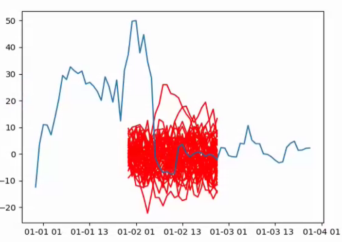
Below is a plot of the samples i get using the code above. As you can see, the samples does not seem to take the previous observations into account. Even though the observations just before the samples are way above zero, the samples start out around zero.

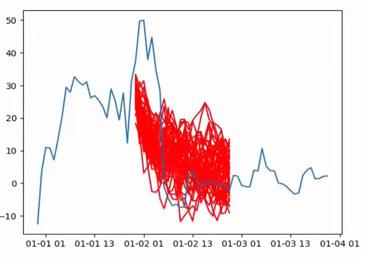
Below is a plot showing an exmaple of what I would like to achieve. The samples takes into account the observations just before the samples are generated, and start out as time series with mean above zero.
I it possible to achive such sampling using the statsmodels package?

Thank you for your help, and please tell me if you need any additional information.

[xiasummer]

I also encountered the same problem. Did you get a breakthrough?

[andrmalm]

I also encountered the same problem. Did you get a breakthrough?

Sorry, I did not. Left this problem a while ago. Still quite interested to achieve something like this in the future though, so will follow this post for updates.

[ChadFulton]

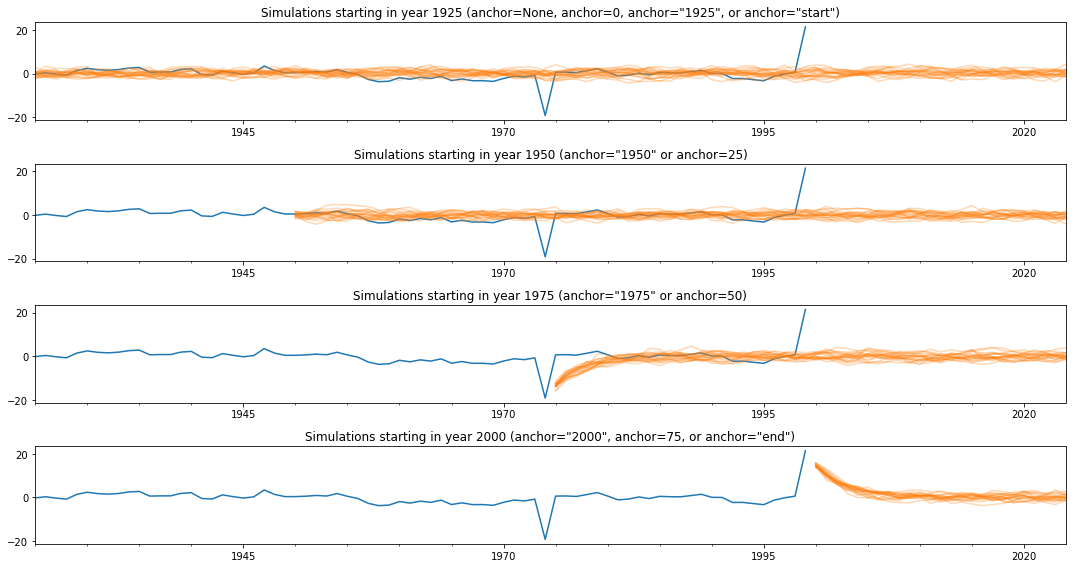
Thanks for reminding me about this. We actually did improve simulation for v0.11 in the PR #6280, but I forgot to come back to this issue.

What we did was to add an anchor keyword argument to simulate that allows you to select which period you want to begin the simulation in. Example follows below:

import numpy as np
import pandas as pd
import statsmodels.api as sm
import matplotlib.pyplot as plt
from scipy.signal import lfilter

np.set_printoptions(suppress=True, precision=8, linewidth=120)

# Simulate some data
nobs = 75
rs = np.random.RandomState(seed=12345)
dta = lfilter([1], [1, -0.7], rs.normal(size=nobs))
endog = pd.Series(dta, index=pd.date_range(start='1925', periods=nobs, freq='AS'))

# Create some outliers
endog.loc['1974'] -= 20
endog.loc['1999'] += 20

# Create the model and evaluate it at the true parameters
mod = sm.tsa.SARIMAX(endog, order=(1, 0, 0))
# phi=0.7
# sigma^2=1.0
res = mod.smooth([0.7, 1.0])
print(res.summary())

# Plot the results of simulations at various anchor periods
fig, axes = plt.subplots(4, figsize=(15, 8))

endog.plot(ax=axes[0])
sim_start = res.simulate(100, repetitions=20)
sim_start.plot(ax=axes[0], color='C1', alpha=0.3, legend=False)
axes[0].set_title('Simulations starting in year 1925 (anchor=None, anchor=0, anchor="1925", or anchor="start")')

endog.plot(ax=axes[1])
sim_25 = res.simulate(75, repetitions=20, anchor='1950')
sim_25.plot(ax=axes[1], color='C1', alpha=0.3, legend=False)
axes[1].set_title('Simulations starting in year 1950 (anchor="1950" or anchor=25)')

endog.plot(ax=axes[2])
sim_50 = res.simulate(50, repetitions=20, anchor='1975')
sim_50.plot(ax=axes[2], color='C1', alpha=0.3, legend=False)
axes[2].set_title('Simulations starting in year 1975 (anchor="1975" or anchor=50)')

endog.plot(ax=axes[3])
sim_end = res.simulate(25, repetitions=20, anchor="2000")
sim_end.plot(ax=axes[3], color='C1', alpha=0.3, legend=False)
axes[3].set_title('Simulations starting in year 2000 (anchor="2000", anchor=75, or anchor="end")')

fig.tight_layout();

And this yields the following figure:

[xiasummer]

Great! This helped a lot!

[ChadFulton]

Great! I'll close this for now as completed, but feel free to re-open or continue the discussion if there is more to be done.