Stars: Reading NetCDF

[michaeldorman]

I am trying to read a NetCDF file (named test3.nc, available on Dropbox here) into R using stars and encounter behavior that seems strange unless I'm missing something.

The file comes from the UERRA regional reanalysis for Europe on single levels from 1961 to present dataset and contains measurements of relative humidity, at a single point in time, over Europe.

The file seems to contain 'lon', 'lat' and 'value' layers, thus representing an irregular grid. Using the raster package, I am able to import these three layers separately and then stack into a multi-band raster, as follows -

library(raster)
lon = raster("test3.nc", varname = "longitude")
lat = raster("test3.nc", varname = "latitude")
z = raster("test3.nc", varname = "r2")
x = stack(lon, lat, z)
x
## class       : RasterStack 
## dimensions  : 1069, 1069, 1142761, 3  (nrow, ncol, ncell, nlayers)
## resolution  : 1, 1  (x, y)
## extent      : 0.5, 1069.5, 0.5, 1069.5  (xmin, xmax, ymin, ymax)
## coord. ref. : NA 
## names       : longitude, latitude, X2.metre.relative.humidity 

I couldn't find a way to get the same information out of the file using stars, however. For example, reading the file with read_stars does not capture the longitude and latitude variables -

library(stars)
r = read_stars("test3.nc")
r
## stars object with 2 dimensions and 1 attribute
## attribute(s), summary of first 1e+05 cells:
##   test3.nc [%]   
##  Min.   : 14.07  
##  1st Qu.: 72.47  
##  Median : 80.32  
##  Mean   : 80.80  
##  3rd Qu.: 89.72  
##  Max.   :100.00  
## dimension(s):
##   from   to offset delta refsys point values    
## x    1 1069     NA    NA     NA    NA   NULL [x]
## y    1 1069     NA    NA     NA    NA   NULL [y]

On the other hand, I don't see a way to specify which variables read_stars is importing. In such case, shouldn't all available variables be read and placed as separate attributes, including longitude and latitude, or am I missing something?

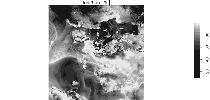
By the way, when using read_stars the array is "upside down" -

plot(r)

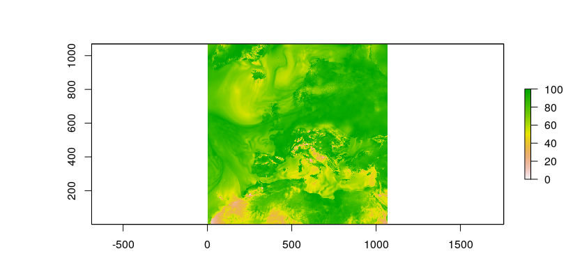
While using raster the orientation is correct -

plot(z)

Also, using the other function read_ncdf gives an error -

r = read_ncdf("test3.nc")
## Error: Unknown NC_TYPE

Thank you very much, will appreciate any help.

[mdsumner]

(I haven't explored the GDAL way much, but it's not behaving how I expect).

In read_ncdf terms, I haven't seen this problem before, in short ncdf4 is reading it but read_ncdf (and tidync that I'm using for an update to read_ncdf) relies on RNetCDF 1.9-1 and it cannot read it. I don't yet know what the issue is.

But, the upcoming release of RNetCDF will be able to read it, or you can install from github: https://github.com/mjwoods/RNetCDF

So with CRAN stars 0.3-1 (only tested on Ubuntu, R 3.6.0):

#devtools::install_github("mjwoods/RNetCDF")
stars::read_ncdf("test3.nc")
stars object with 2 dimensions and 3 attributes
attribute(s), summary of first 1e+05 cells:
     r2 [%]         latitude [°]   longitude [°]
 Min.   :  9.797   Min.   :20.29   Min.   :  0.0001
 1st Qu.: 47.189   1st Qu.:23.86   1st Qu.: 13.6192
 Median : 60.449   Median :25.06   Median : 26.9819
 Mean   : 62.653   Mean   :25.05   Mean   :135.7698
 3rd Qu.: 80.396   3rd Qu.:26.37   3rd Qu.:346.9164
 Max.   :100.000   Max.   :28.65   Max.   :359.9990
dimension(s):
  from   to offset delta refsys point values
x    1 1069    0.5     1     NA    NA   NULL [x]
y    1 1069    0.5     1     NA    NA   NULL [y]

In an upcoming release of stars I'm hoping to make the interpretation better. Thanks for the example!

[michaeldorman]

Great, I used install_github("mjwoods/RNetCDF") and now read_ncdf works for me and gives the same output you got. Thank you very much!

[edzer]

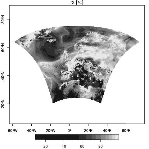
Your data are on a curvilinear grid, cover the zero meridian, and the creators thought it was a clever idea to have longitude range from 0 to 360 instead of the somewhat more usual -180 to 180. Hence, this rather ugly hack to read & plot:

library(stars)
r = read_ncdf("test3.nc", curvilinear = c("longitude", "latitude"))
lo = units::drop_units(r$longitude)
lo[lo > 180] = lo[lo > 180] - 360 # rescale to -180,180
attr(r, "dimensions")[["x"]]$values = lo
plot(r, border = NA, axes = TRUE)

[michaeldorman]

I noticed the longitude issue - your solution is very helpful, thanks a lot!

My attempt was this -

r$longitude[r$longitude > set_units(180, "degrees")] = 
  r$longitude[r$longitude > set_units(180, "degrees")] - 
  set_units(360, "degrees")

This seems to modify the values but has no effect on plot, I have more to learn about how curvilinear grids work in general and in stars :-)

[edzer]

Your solution to recompute longitude is of course much more elegant and fool-proof!

The reason why changing longitude does not change the plotting is that r$longitude is a cube attribute, not a dimension value / array: suppose you had a time series of r2 (you actually do, but with a single time instance), then all arrays in it need to have identical dimensions; longitude and latitude however would not change over time, and would no longer fit as attributes.

[michaeldorman]

A different issue with the same ECMWF product: when the NetCDF file contains more than one point in time, as.data.frame loses the time dimension. (Another minor inconvenience is that the time dimension format is interpreted as numeric rather than one of the time formats.)

Here is a reproducible example reading a NetCDF file from Dropbox:

# Read NetCDF file
library(stars)
url = "https://www.dropbox.com/s/9xuhacw1ieiyrw5/era_TEST.nc?dl=1"
tmp = tempfile(fileext = ".nc")
download.file(url, tmp)
r = read_ncdf(tmp, curvilinear = c("longitude", "latitude"))

## no 'var' specified, using r2

## other available variables:
##  time, step, heightAboveGround, latitude, longitude, valid_time

## Warning in attribute$variable == var: longer object length is not a
## multiple of shorter object length

## Warning in .get_nc_projection(meta$attribute, rep_var, all_coord_var): No
## projection information found in nc file.

# Normalize x-coordinates
x = st_get_dimension_values(r, "x")
x[x > 180] = x[x > 180] - 360
attributes(r)$dimensions$x$values = x

The summary looks fine, other than the fact that time is numeric:

# Summary
r

## stars object with 3 dimensions and 1 attribute
## attribute(s), summary of first 1e+05 cells:
##      r2 [%]      
##  Min.   : 8.806  
##  1st Qu.:38.357  
##  Median :53.406  
##  Mean   :52.836  
##  3rd Qu.:69.064  
##  Max.   :98.152  
## dimension(s):
##      from   to     offset delta                       refsys point
## x       1 1069         NA    NA +proj=longlat +datum=WGS8...    NA
## y       1 1069         NA    NA +proj=longlat +datum=WGS8...    NA
## time    1    4 1517173200 21600                           NA    NA
##                                values    
## x    [1069x1069] -58.1048,...,74.1044 [x]
## y      [1069x1069] 20.292,...,75.3465 [y]
## time                             NULL    
## curvilinear grid

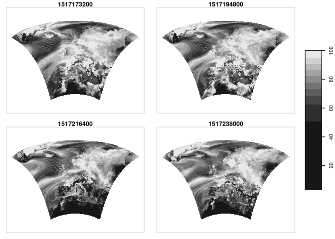
The plot also seems correct:

# Plot
plot(r)

Converting to data.frame, however, loses the time dimension for some reason:

# Converting to 'data.frame': 'time' column is missing...
dat = as.data.frame(r)
head(dat)

##           x        y           r2
## 1 -17.48600 20.29200 78.16563 [%]
## 2 -17.44187 20.30666 78.02110 [%]
## 3 -17.39773 20.32130 77.87657 [%]
## 4 -17.35357 20.33591 77.75352 [%]
## 5 -17.30939 20.35051 77.66954 [%]
## 6 -17.26519 20.36508 77.62852 [%]

My workaround was to convert to sf with st_as_sf(r, as_points=TRUE), re-calculate the x and y columns from the geometry, then drop the geometry. Just in case I'm missing something, will be happy to hear any suggestion. Thanks!

[michaeldorman]

Great, thank you very much! It works now:

library(stars)
url = "https://www.dropbox.com/s/9xuhacw1ieiyrw5/era_TEST.nc?dl=1"
tmp = tempfile(fileext = ".nc")
download.file(url, tmp)
r = read_ncdf(tmp, curvilinear = c("longitude", "latitude"))
x = st_get_dimension_values(r, "x")
x[x > 180] = x[x > 180] - 360
attributes(r)$dimensions$x$values = x
dat = as.data.frame(r)
head(dat)

##           x        y       time           r2
## 1 -17.48600 20.29200 1517173200 78.16563 [%]
## 2 -17.44187 20.30666 1517173200 78.02110 [%]
## 3 -17.39773 20.32130 1517173200 77.87657 [%]
## 4 -17.35357 20.33591 1517173200 77.75352 [%]
## 5 -17.30939 20.35051 1517173200 77.66954 [%]
## 6 -17.26519 20.36508 1517173200 77.62852 [%]

[edzer]

Thanks for bringing this up!

[michaeldorman]

Sorry, another issue with the same dataset, regarding the "time" dimension values.

The time stamps read using read_stars are correct and match the time stamps specified when downloading this sample file:

import cdsapi
c = cdsapi.Client()
c.retrieve(
'reanalysis-uerra-europe-single-levels',
{
    'format':'netcdf',
    'origin':'mescan_surfex',
    'variable':'2m_relative_humidity',
    'year':'2018',
    'month':'01',
    'day':'01',
    'month':'01',
    'day':'29',
    'time':['00:00','06:00','12:00','18:00'],
    'format': 'netcdf'
},
'era_TEST.nc')

Here is a reproducible example:

library(stars)

# Get NetCDF file
url = "https://www.dropbox.com/s/9xuhacw1ieiyrw5/era_TEST.nc?dl=1"
tmp = tempfile(fileext = ".nc")
download.file(url, tmp)

# Read using 'read_stars'
r = read_stars(tmp, curvilinear = c("longitude", "latitude"))
st_get_dimension_values(r, "time")

## [1] "2018-01-29 00:00:00 UTC" "2018-01-29 06:00:00 UTC"
## [3] "2018-01-29 12:00:00 UTC" "2018-01-29 18:00:00 UTC"

However, when reading the same file with read_ncdf, the times are shifted 3hr backwards:

# Read using 'read_ncdf'
r = read_ncdf(tmp, curvilinear = c("longitude", "latitude"))
st_get_dimension_values(r, "time") %>% 
  as.POSIXct(origin = as.POSIXct("1970-01-01T00:00:00+00:00", tz = "UTC"), tz = "UTC")

## [1] "2018-01-28 21:00:00 UTC" "2018-01-29 03:00:00 UTC"
## [3] "2018-01-29 09:00:00 UTC" "2018-01-29 15:00:00 UTC"

Since the values are numeric they need to be converted with as.POSIXct, relying on the origin as specified in the gdal_metadata(tmp):

gdal_metadata(tmp)[49]

## [1] "time#units=seconds since 1970-01-01T00:00:00+00:00"

Interestingly, however, the metadata includes different numeric values for seconds since "origin". Using those gives the expected times, just like the ones readily available with st_read_stars:

gdal_metadata(tmp)[10]

## [1] "NETCDF_DIM_time_VALUES={1517184000,1517205600,1517227200,1517248800}"

c(1517184000,1517205600,1517227200,1517248800) %>% 
  as.POSIXct(origin = as.POSIXct("1970-01-01T00:00:00+00:00", tz = "UTC"), tz = "UTC")

## [1] "2018-01-29 00:00:00 UTC" "2018-01-29 06:00:00 UTC"
## [3] "2018-01-29 12:00:00 UTC" "2018-01-29 18:00:00 UTC"

My question is whether this is a bug in st_read_ncdf, particularly in the way that this function gets the time values from the metadata? Or am I missing something in the time handling in this format?

Thank you very much for any help!

[edzer]

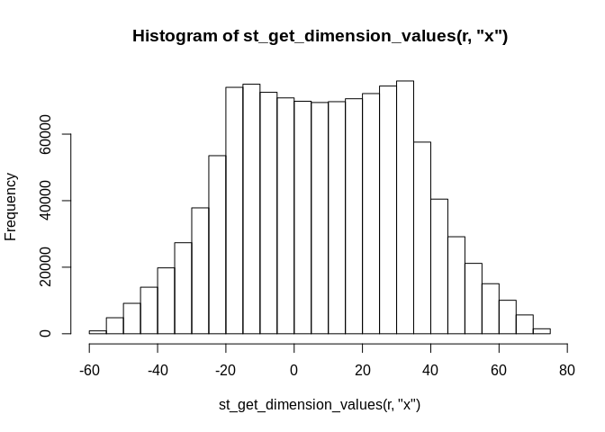
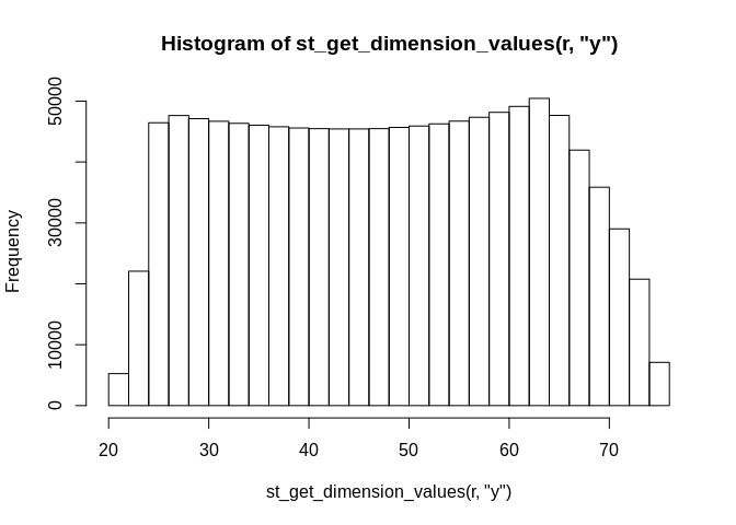
There's much more funny going on with this dataset: try plotting it, look at the x and y dimension values.

[michaeldorman]

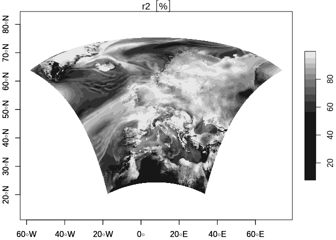
Thanks for looking into this. Not sure I understand what you mean, the x and y dimensions look fine to me:

library(stars)

# Read NetCDF file
url = "https://www.dropbox.com/s/9xuhacw1ieiyrw5/era_TEST.nc?dl=1"
tmp = tempfile(fileext = ".nc")
download.file(url, tmp)
r = read_ncdf(tmp, curvilinear = c("longitude", "latitude"))
x = st_get_dimension_values(r, "x")
x[x > 180] = x[x > 180] - 360
attributes(r)$dimensions$x$values = x

# Dimension values
hist(st_get_dimension_values(r, "x"))

hist(st_get_dimension_values(r, "y"))

# Plot
plot(r[,,,1], axes = TRUE)