Seurat: average expression, dot plot and violin plot

[Tushar-87]

Hello @satijalab @mojaveazure and everyone else using visualization functions,

I am posting the following problems after doing keyword search in issue section.

The problem is discrepancy between average expression of a gene and visualization tools namely Violin plot and dot plot.

I calculated average expression of a gene using:
AverageExpression(ec.true, assays = "RNA", slot = "data", add.ident = "orig.ident", features = "Itgb1")

The results are:
$RNA
wt2cx_wt2cx a4cx_a4cx wt2bm_wt2bm a4bm_a4bm
Itgb1 3.548707 3.222106 3.530166 3.246126
(there are four idents)
I also obtained fold change using findmarker function.
> ec.de.cx.a4wt.pseudo0 <- FindMarkers(ec.true, ident.1 = "a4cx", ident.2 = "wt2cx", min.pct = 0, logfc.threshold = 0, pseudocount.use = 0)
As expected, fold change obtained here is in agreement with average expression values calculated using average expression function.
itgb1 dot plot.pdf
vln itgb1.pdf

Then I made violin plot with following code:
> VlnPlot(ec.true, features = "Itgb1", assay = "RNA", slot = "data", pt.size = 0.05)
Please find the attached violin plot,

Then I made dot plot:
> DotPlot(ec.true, features = "Itgb1", scale.max = 100, scale.min = 0, col.max = 5, col.min = 0, dot.scale = 7, assay = "RNA") + RotatedAxis()

Also find the attached dot plot.

1) The calculated average expression value is different from dot plot and violin plot. Also the two plots differ in apparent average expression values (In violin plot, almost no cell crosses 3.5 value although the calculated average value is around 3.5). Same assay was used for all these operations.
2) In dot plot, the difference in average expression between two groups appears exaggerated after considering violin plot and calculated values.

Kindly help me to understand these apparent discrepancies.

[liuxl18-hku]

I think DotPlot using scaled (z-score) of data used in VlnPlot: https://github.com/satijalab/seurat/blob/94343c4fdb35a3a1e7a7e14d4a0bb0cec657075c/R/visualization.R#L1993

That's why you see the exaggeration and also may not be correct to use asymmetric col.min and col.max

bless~

[Tushar-87]

@liuxl18-hku thanks. Even one considers scaling, the kind of difference we see in dot plot simiply appears unrealistic. I have tried symmetric col min and max values, for example -1 to 1 or -2 to 2. The exaggerated differences between groups still exist. The actual difference is meagre 8%. The dot plot shows drastic difference. Also, the scale bar for expression denotes negative values which are difficult to explain.
Moreover, this does not explain the discrepancy between vln plot and calculated values using averageExpression function. When no cell in vln plot crosses 3.5 value, how can caculated average expression be around 3.5?

[liuxl18-hku]

@Tushar-87 ,

Very critical thinking. Let me try to explain.

First, why the output of AverageExpression() looks different with VlnPlot()

As we know that data slot contains log-scaled data. What AE() did was (in your case with use.scale = FALSE and use.raw = FALSE):

mean(x = expm1(x = x))

Means that the output is NOT in log-scale anymore (Pls refer to #758)

However, what VP() used for y-axis "Expression Level", I think, is the log-scaled value (log1p, I think). So if you try to take logarithm of your AE() output:

> log1p(c(3.548707,3.222106,3.530166,3.246126))
[1] 1.514843 1.440334 1.510759 1.446007

Actually they are consistent with the VlnPlot.

Second, z-score like scaling (R function: base::scale() can introduce big exaggeration (using your average expression again)

> scale(c(3.548707,3.222106,3.530166,3.246126))
           [,1]
[1,]  0.9163561
[2,] -0.9318587
[3,]  0.8114337
[4,] -0.7959310
attr(,"scaled:center")
[1] 3.386776
attr(,"scaled:scale")
[1] 0.1767116

After applying your settings of col.min = 0 and col.max = 5, the scaled values will become:

           [,1]
[1,]  0.9163561
[2,] 0 # -0.9318587 < 0,  use 0
[3,]  0.8114337
[4,] 0 # -0.7959310 < 0, use 0

That's actually what Seurat used (if I am not wrong, based on my understanding of the DotPlot() code) for coloring the dotplot. That's why you saw the two groups "a4bm" and "a4cx" looks so different (in scaled space) with the other two groups with positive values.

bless~

[Tushar-87]

@liuxl18-hku Thanks a lot for your clear explanation!!
Your arguement that vln plots have log scaled values makes sense. It will be great if @mojaveazure or @satijalab could confirm this.
I see the problem with dot plot using z -score like scaling. Is there any way to mitigate this? For example changing the parameters in code? I tried to play around with col min and col max with no success so far...

[liuxl18-hku]

@Tushar-87 ,

Here is a very crude way to get around, but better to wait developer's confirmation.

I tested it on the public pbmc3k dataset.

# devtools::install_github('satijalab/seurat-data');
library(SeuratData)
# InstallData("pbmc3k")
data("pbmc3k") # pbmc3k

pbmc3k <- NormalizeData(pbmc3k, normalization.method = "LogNormalize", scale.factor = 10000)
pbmc3k <- pbmc3k[, !is.na([email protected]$seurat_annotations)]
Idents(pbmc3k) <- [email protected]$seurat_annotations

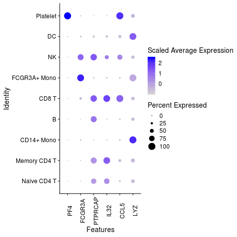
features.plot <- c("LYZ", "CCL5", "IL32", "PTPRCAP", "FCGR3A", "PF4")
DotPlot(object = pbmc3k, features = features.plot, assay="RNA") + 
    guides(color = guide_colorbar(title = 'Scaled Average Expression')) + 
    theme(axis.text.x = element_text(angle=90))

# very add-hoc solution
# ideas from mnel's post in https://stackoverflow.com/questions/13407236/remove-a-layer-from-a-ggplot2-chart

library(ggplot2)
features.plot <- c("LYZ", "CCL5", "IL32", "PTPRCAP", "FCGR3A", "PF4")
g <- DotPlot(object = pbmc3k, features = features.plot, assay="RNA")

# > g$layers
# [[1]]
# mapping: size = ~pct.exp, colour = ~avg.exp.scaled 
# geom_point: na.rm = FALSE
# stat_identity: na.rm = FALSE
# position_identity 

# > g$data
#              avg.exp   pct.exp features.plot     id avg.exp.scaled
# LYZ     3.303911e+79 60.407407           LYZ pbmc3k            NaN
# CCL5    1.707925e+25 31.925926          CCL5 pbmc3k            NaN
# IL32    3.126373e+23 55.407407          IL32 pbmc3k            NaN
# PTPRCAP 1.608967e+12 64.037037       PTPRCAP pbmc3k            NaN
# FCGR3A  8.475464e+07 18.407407        FCGR3A pbmc3k            NaN
# PF4     3.125317e+23  1.592593           PF4 pbmc3k            NaN

g$layers[[1]] <- NULL # remove original geom_point layer where the color scale is hard-coded to use scaled average expression
g <- g + 
    geom_point(mapping = aes_string(size = 'pct.exp', color = 'avg.exp')) +
    guides(color = guide_colorbar(title = 'Average Expression')) + 
    theme(axis.text.x = element_text(angle=90))

plot(g)

[timoast]

@liuxl18-hku is correct that the DotPlot shows scaled data, while VlnPlot shows the normalized data. This accounts for the differences you see.

As stated here, we use the scaled data for DotPlot so that we can visualize highly and lowly expressed genes on the same color scale.

[YiweiNiu]

@timoast Hi, sometimes only a subset of genes (e.g. highly variable features) was used to compute scale.data to speed up the calculation. In this case, how does DotPlot handle genes that were not in the scale.data slot?