Seurat: Set the X axis for FeaturePlot

[lvila]

I am trying to use FeaturePlot to show the difference in a gene between a control and a mutant (in different plots). The problem is that the control X axis is from -50 to 50, and the mutant starts at -20. I would like to set the x axis value to make it comparable but xlim doesn't work. Is there a way to do this?

[ShanSabri]

Would you mind posting the output tSNE plot for each FeaturePlot? Are these two separate tSNE embeddings?

[lvila]

These are two separate tSNE plots featuring a gene. I am just showing the same gene on each one of them to compare them. Top is control and bottom is mutant. The x axis have different values that I haven't been able to change.

[ShanSabri]

But if they are two completely different embeddings then why would you want to extend out the x-axis? By default the full embedding is centered to the plot. Expanding the limits of the axis will not show additional data. To be clear, tSNE plots aren't easily interpretable in terms of the axes/units of the original, high-dimensional data. So I wouldn't try to interpret a tSNE plot quantitatively; t-SNE is just a visualization technique, nothing more.

[lvila]

Yes, but to show a control and a mutant and be comparable I would need to show that whatever population the control has at -50 is not in the mutant. The absence of that population is the reason why the mutant axis starts at -20. That's why I am trying to set the value of x and make it the same.

For example, I was able to do this with the TSNEPlot function:

TSNEPlot(ctrl.subset, do.return=TRUE) + xlim (c(-50, 50))
TSNEPlot(mut.subset, do.return=TRUE) + xlim (c(-50, 50))

[ShanSabri]

I would need to show that whatever population the control has at -50 is not in the mutant.

tSNE is stochastic. If these are really two completely independent embeddings then there is no reason to assume that the same population found in both embeddings will lie in the same position. In fact, it is highly unlikely.

[lvila]

They are not completely independent. The original file is an aggregate file and I separated them with SubsetData. So the tSNE actually lines up.

[mojaveazure]

Have you tried coord_cartesian instead of xlim? It's similar, but operates differently so I think it'll work better. Also try FeatureHeatmap, setting the group.by argument to the metadata column differentiating between your mutants and controls.

[lvila]

I think the problem is that FeaturePlot is not returning a ggplot2 so I can't use those arguments. For example, if I try:

FeaturePlot(object = mut.subset,
            features.plot = "gene1",
            cols.use = c("grey", "blue"), do.return = TRUE,
            reduction.use = "tsne") + xlim (c(-50, 50))

It returns as NULL.

If I do it inside the FeaturePlot:

FeaturePlot(object = mut.subset,
            features.plot = "gene1",
            cols.use = c("grey", "blue"), do.return = TRUE,
            reduction.use = "tsne", coord_cartesian(xlim = c(-50, 50)))

it throws an error:

Error in .subset2(x, name) : 
  wrong arguments for subsetting an environment

Trying the same thing using xlim as an argument to FeaturePlot:

FeaturePlot(object = mut.subset,
            features.plot = "gene1",
            cols.use = c("grey", "blue"), do.return = TRUE,
            reduction.use = "tsne", xlim = c(-50, 50))

also throws an error:

Error in FeaturePlot(object = mut.subset, features.plot = "gene1",  : 
  unused argument (xlim = c(-50, 50))

[lvila]

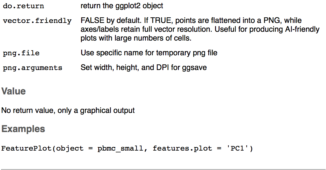
It's confusing because it says you can use the do.return argument but in value it says it's only a graphical output. I think this is why the arguments used to modify the ggplot2 that for example work with TSNEPlot, don't work with FeaturePlot.

[lvila]

I looked at the source code for FeaturePlot and found that it doesn't actually return a ggplot2 object directly; instead it returns a _list_ of ggplot2 objects. The following code works as expected:

plist <- FeaturePlot(object = mut.subset,
            features.plot = c("gene1", "gene2","gene3"),
            cols.use = c("grey", "blue"), do.return = TRUE,
            reduction.use = "tsne")

plist[[1]] + xlim(c(-50,50))

[mjdapper]

I know v3 is quite new but I'm having a similar problem with keeping axes fixed when splitting out and none of the above solutions worked. Any ideas?

[andrewwbutler]

Hi,

One way to achieve this in v3 is as follows:

plots <- FeaturePlot(object = pbmc_small, features = rownames(pbmc_small)[1:6], combine = FALSE)
# replace arguments in xlim and ylim with the fixed limits you want
plots <- lapply(X = plots, FUN = function(p) p + xlim(c(0, 25)) + ylim(c(-25, 0)))
CombinePlots(plots = plots)

Alternative, we've found the patchwork package to be quite useful for this sort of thing too, although it's not on CRAN yet.

plots <- FeaturePlot(object = pbmc_small, features = rownames(pbmc_small)[1:6], combine = FALSE)
patchwork::wrap_plots(plots) * xlim(c(0, 50))