Python-binance: get MACD and Moving Averages (so that they are the same as those plotted by Binance)?
is there a way to obtain MACD and moving averages?
 DaniZz
All 14 comments
You need to calculate them yourself
 Rob-bb
on 17 Feb 2018
Rob-bb
on 17 Feb 2018
I guessed so :)
I found this post as inspiration. If people are interested I can post here my functions computing MAs on the tickers
DaniZz
on 18 Feb 2018
still struggling with computing MACD, it doesn't give the same result as Binance...
can anyone help?
here's my code:
`
import numpy as np
import matplotlib.pyplot as plt
###### data
prices = np.array([ 0.00061422, 0.00061422, 0.00061593, 0.00061672, 0.0006161 ,
0.00061233, 0.000615 , 0.00061305, 0.00061346, 0.00061417,
0.00061428, 0.00061418, 0.0006115 , 0.00061203, 0.0006125 ,
0.00061295, 0.00061296, 0.00061295, 0.00061242, 0.00061144,
0.00060874, 0.00060661, 0.00060512, 0.00060931, 0.000611 ,
0.0006129 , 0.00061296, 0.000613 , 0.00061138, 0.0006115 ,
0.0006123 , 0.0006123 , 0.00061288, 0.00061494, 0.000615 ,
0.0006146 , 0.00061488, 0.00061399, 0.00061285, 0.0006129 ,
0.0006129 , 0.00061291, 0.0006134 , 0.00061338, 0.00061355,
0.0006139 , 0.00061475, 0.0006167 , 0.0006158 , 0.000617 ,
0.00061638, 0.00061452, 0.0006164 , 0.00061641, 0.00061646,
0.00061898, 0.0006198 , 0.00061818, 0.00061922, 0.00061979,
0.00061977, 0.00061924, 0.00061626, 0.00061488, 0.000616 ,
0.000616 , 0.00061693, 0.0006165 , 0.0006165 , 0.00061699,
0.00061685, 0.00061687, 0.00061691, 0.000617 , 0.00061784,
0.00061899, 0.0006177 , 0.000617 , 0.00061732, 0.0006176 ,
0.0006174 , 0.00061739, 0.00061739, 0.00061794, 0.0006185 ,
0.0006185 , 0.00061785, 0.00061735, 0.00061743, 0.00061742,
0.00061429, 0.0006152 , 0.00061451, 0.00061514, 0.0006143 ,
0.000614 , 0.0006154 , 0.0006148 , 0.00061444, 0.00061572])
###### functions
def moving_average(x, n, type='simple'):
"""
compute an n period moving average.
type is 'simple' | 'exponential'
"""
x = np.asarray(x)
if type == 'simple':
weights = np.ones(n)
else:
weights = np.exp(np.linspace(-1., 0., n))
weights /= weights.sum()
a = np.convolve(x, weights, mode='full')[:len(x)]
a[:n] = a[n]
return a
def relative_strength(prices, n=14):
"""
compute the n period relative strength indicator
http://stockcharts.com/school/doku.php?id=chart_school:glossary_r#relativestrengthindex
http://www.investopedia.com/terms/r/rsi.asp
"""
deltas = np.diff(prices)
seed = deltas[:n+1]
up = seed[seed >= 0].sum()/n
down = -seed[seed < 0].sum()/n
rs = up/down
rsi = np.zeros_like(prices)
rsi[:n] = 100. - 100./(1. + rs)
for i in range(n, len(prices)):
delta = deltas[i - 1] # cause the diff is 1 shorter
if delta > 0:
upval = delta
downval = 0.
else:
upval = 0.
downval = -delta
up = (up*(n - 1) + upval)/n
down = (down*(n - 1) + downval)/n
rs = up/down
rsi[i] = 100. - 100./(1. + rs)
return rsi
def moving_average_convergence(x, nslow=26, nfast=12):
"""
compute the MACD (Moving Average Convergence/Divergence) using a fast and slow exponential moving avg'
return value is emaslow, emafast, macd which are len(x) arrays
"""
emaslow = moving_average(x, nslow, type='exponential')
emafast = moving_average(x, nfast, type='exponential')
return emaslow, emafast, emafast - emaslow
###### code
nslow = 26
nfast = 12
nema = 9
emaslow, emafast, macd = moving_average_convergence(prices, nslow=nslow, nfast=nfast)
ema9 = moving_average(macd, nema, type='exponential')
rsi = relative_strength(prices)
wins = 80
plt.figure(1)
### prices
plt.subplot2grid((8, 1), (0, 0), rowspan = 4)
plt.plot(prices[-wins:], 'k', lw = 1)
### rsi
plt.subplot2grid((8, 1), (5, 0))
plt.plot(rsi[-wins:], color='black', lw=1)
plt.axhline(y=30, color='red', linestyle='-')
plt.axhline(y=70, color='blue', linestyle='-')
## MACD
plt.subplot2grid((8, 1), (6, 0))
plt.plot(ema9[-wins:], 'red', lw=1)
plt.plot(macd[-wins:], 'blue', lw=1)
plt.subplot2grid((8, 1), (7, 0))
plt.plot(macd[-wins:]-ema9[-wins:], 'k', lw = 2)
plt.axhline(y=0, color='b', linestyle='-')
plt.show()
`


DaniZz
on 20 Feb 2018
EMA and MA are similar but different beasts. I had problems when I was using my own function (also using np) then I switched to using TALIB's ema function and now mine match the binance macd.
Rob-bb
on 20 Feb 2018
HA! I wish I had read that this morning :D
I tried talib and that gives what I want :)

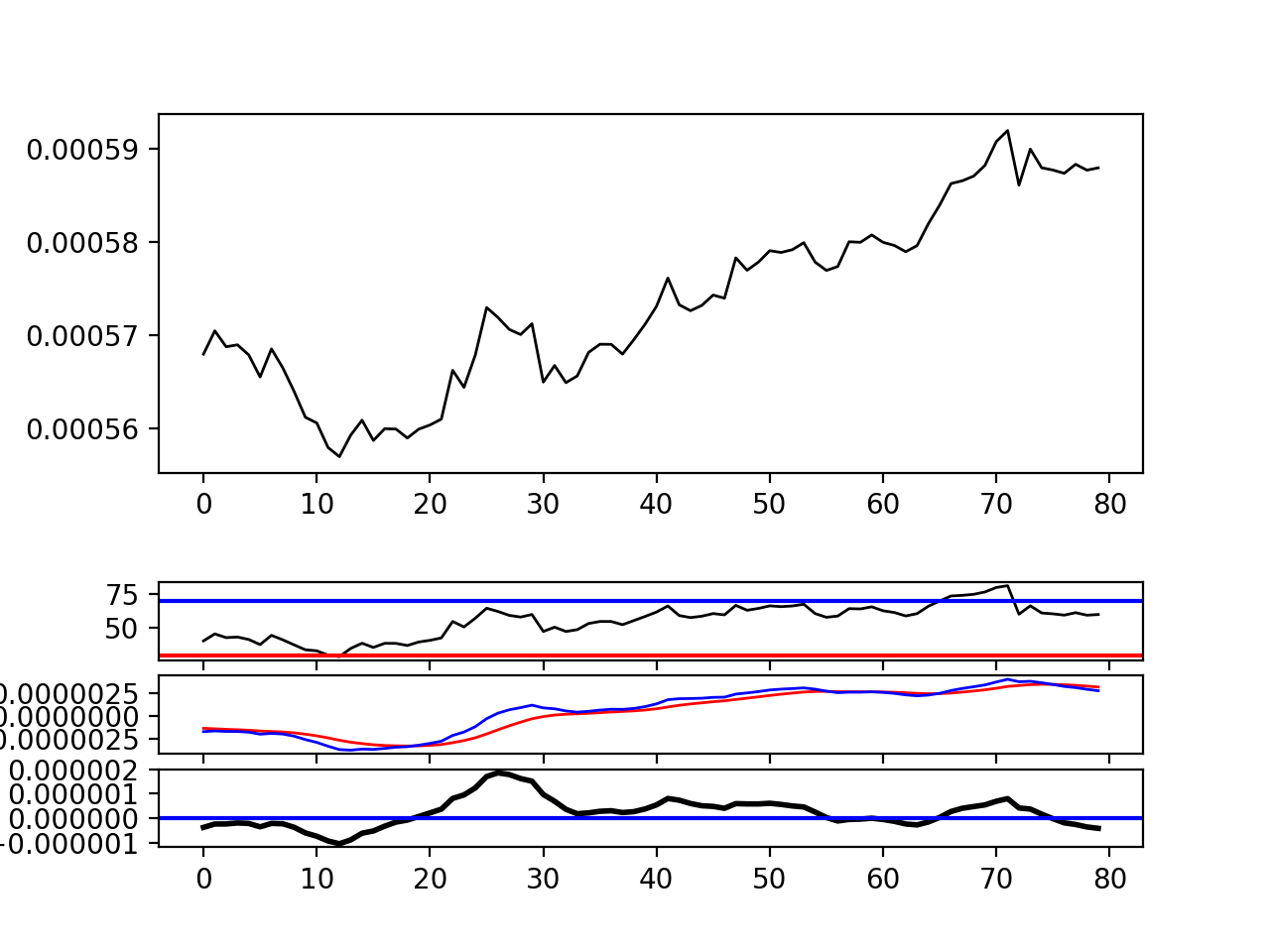
I guess they are two different ways to compute the MACD (but I tried non-exponential average before and did not work anyway, so I still don't know the reason underlying the difference).
import talib
macd, macdsignal, macdhist = talib.MACD(prices, fastperiod=12, slowperiod=26, signalperiod=9)
@DaniZz - I would appreciate it of you could post your code for your TA-Lib example.
I've been struggling to find an example for noobs of using python-binance websockets data with TA-Lib.
Would be grateful if you had time to post an example, if you have one to hand.
 rootscript
on 5 Mar 2018
rootscript
on 5 Mar 2018
may I know what is wins? why it is 80?
 syuhaida31
on 10 May 2018
syuhaida31
on 10 May 2018
@rootscript and @syuhaida31
sorry I haven't worked on these scripts for a couple of months and I haven't had time to post some workable examples.
I promise I will post this code ASAP. It is just an adaption from a Matplotlib template (which I can't find right now)
@syuhaida31 80 is the number of time points (80 minutes)
DaniZz
on 14 May 2018
is it default to 80 or I have to determine my own time points?
syuhaida31
on 15 May 2018
try this, not sure it works right away :)
import numpy as np

import matplotlib.pyplot as plt
import talib
import matplotlib.font_manager as font_manager
from matplotlib import collections  as mc

###### CLASS SANDWICH
#### CONTAINS arrays with different info for every time point
### price, ups, downs, open, close, vol, and indexes like MACD, RSI  and increments

class Sw (object):

    def __init__ (self, candles = None, **kwargs):

        if candles:
            # imported values
            self.open =  np.array([float(x[1]) for x in candles])
            self.high = np.array([float(x[2]) for x in candles])
            self.low = np.array([float(x[3]) for x in candles])
            self.close = np.array([float(x[4]) for x in candles])
            self.volume = np.array([float(x[5]) for x in candles])


        # computes the inedexes

            #classic
            self.rsi = talib.RSI(self.close)
            self.macd, self.macdsignal, uaua   = talib.MACD(self.close, fastperiod=12, slowperiod=26, signalperiod=9)
            self.rocp = talib.ROCP(self.close)

            # overlap
            self.sar = talib.SAR(self.high, self.low)

            '''
            self.kama = talib.KAMA(self.close)
            self.bb_up, self.bb_mid, self.bb_low = talib.BBANDS(self.close)

            # momentum
            self.arosc = talib.AROONOSC(self.high, self.low)
            self.mom = talib.MOM(self.close)
            self.slostok, self.slostod = talib.STOCH(self.high, self.low, self.close)
            self.fasstok, self.fasstod = talib.STOCHF(self.high, self.low, self.close)

            self.ulto = talib.ULTOSC(self.high, self.low, self.close)
            self.wilr = talib.WILLR(self.high, self.low, self.close)
            self.trix = talib.TRIX(self.close)

            # vol
            self.chaos = talib.ADOSC(self.high, self.low, self.close, self.volume)
            self.obv = talib.OBV(self.close, self.volume)

            # cycle
            self.hilper = talib.HT_DCPERIOD(self.close)
            self.hilpha = talib.HT_DCPHASE(self.close)
            self.phasorin, self.phasorquad  = talib.HT_PHASOR(self.close)
            #self.hilsine = talib.HT_SINE(self.close) # gives out of range error
            self.hiltrend = talib.HT_TRENDMODE(self.close)

            '''


def plotSerie (serie, trades = None, coin = None, wins = None, timeframe = "1min", numberfig = 1, **kwargs):


    if not wins:
        wins = len(serie)


    prices = serie.close
    rsi = serie.rsi
    macd = serie.macd
    macdsignal = serie.macdsignal
    sar = serie.sar


    ##################################

    plt.rc('axes', grid=True)
    plt.rc('grid', color='0.75', linestyle='-', linewidth=0.5)

    textsize = 9
    left, width = 0.1, 0.8
    rect1 = [left, 0.7, width, 0.2]
    rect2 = [left, 0.3, width, 0.4]
    rect3 = [left, 0.1, width, 0.2]


    fig = plt.figure(numberfig, facecolor='white')
    axescolor = '#f6f6f6'  # the axes background color

    ax1 = fig.add_axes(rect1, axisbg=axescolor)  # left, bottom, width, height
    ax2 = fig.add_axes(rect2, axisbg=axescolor, sharex=ax1)
    ax2t = ax2.twinx()
    ax3 = fig.add_axes(rect3, axisbg=axescolor, sharex=ax1)


    fillcolor = 'purple'

    ax1.plot(rsi[-wins:], color=fillcolor)
    ax1.axhline(70, color=fillcolor)
    ax1.axhline(30, color=fillcolor)

    ax1.axhline(50, lw=0.5)

    #ax1.fill_between(rsi, 70, where=(rsi >= 70), facecolor=fillcolor, edgecolor=fillcolor)
    #ax1.fill_between(rsi, 30, where=(rsi <= 30), facecolor=fillcolor, edgecolor=fillcolor)
    ax1.text(0.6, 0.9, '>70 = overbought', va='top', transform=ax1.transAxes, fontsize=textsize)
    ax1.text(0.6, 0.1, '<30 = oversold', transform=ax1.transAxes, fontsize=textsize)
    ax1.set_ylim(0, 100)
    ax1.set_yticks([30, 70])
    ax1.text(0.025, 0.95, 'RSI (14)', va='top', transform=ax1.transAxes, fontsize=textsize)
    ax1.set_title('%s,  %s interval' % (coin, timeframe))


    # plot the price and volume data
    '''
    dx = r.adj_close - r.close
    low = r.low + dx
    high = r.high + dx

    deltas = np.zeros_like(prices)
    deltas[1:] = np.diff(prices)
    up = deltas > 0
    ax2.vlines(r.date[up], low[up], high[up], color='black', label='_nolegend_')
    ax2.vlines(r.date[~up], low[~up], high[~up], color='black', label='_nolegend_')
    '''


    ma20 = moving_average(prices[-wins:], 20, type='simple')
    #ma200 = moving_average(prices, 200, type='simple')

    linema20, = ax2.plot(ma20, color='orange', lw=1, label='MA (20)')

    lineprice = ax2.plot(prices[-wins:], color='red', lw=1.5, label='price')
    if trades:

        lines_start = [(x.ixstart, x.prices[0]) for x in trades if x.coin == coin]
        lines_end = [(x.ixend, x.prices[-1]) for x in trades if x.coin == coin]

        lines = zip(lines_start, lines_end)

        lc = mc.LineCollection(lines, colors="b", linewidths=3, label='trades')
        ax2.add_collection(lc)
        #ax2.autoscale()
        #ax2.margins(0.1)

        # plot profit

        netprof = sum([x.netprof for x in trades])
        ntrades = sum([len(x.prices)-1 for x in trades])

        ttext = " trade intervals= %s\n net profit= %s perc" % (str(ntrades), str(round(netprof, 1)) )
        #print ttext


        ax2.text(len(prices) - len(prices)/5, max(prices) - max(prices)/30, ttext, fontsize = 10)


    #### OTHER INDICATORS

    ax2.plot(sar, "o", color='y', lw=0.3, mfc='none', label='SAR')


    #linema200, = ax2.plot(r.date, ma200, color='red', lw=2, label='MA (200)')

    '''
    last = r[-1]
    s = '%s O:%1.2f H:%1.2f L:%1.2f C:%1.2f, V:%1.1fM Chg:%+1.2f' % (
        today.strftime('%d-%b-%Y'),
        last.open, last.high,
        last.low, last.close,
        last.volume*1e-6,
        last.close - last.open)
    t4 = ax2.text(0.3, 0.9, s, transform=ax2.transAxes, fontsize=textsize)
    '''

    props = font_manager.FontProperties(size=10)
    leg = ax2.legend(loc='center left', shadow=True, fancybox=True, prop=props)
    leg.get_frame().set_alpha(0.5)

    '''

    volume = (r.close*r.volume)/1e6  # dollar volume in millions
    vmax = volume.max()
    poly = ax2t.fill_between(r.date, volume, 0, label='Volume', facecolor=fillcolor, edgecolor=fillcolor)
    ax2t.set_ylim(0, 5*vmax)
    ax2t.set_yticks([])

    '''

    #ax3.plot(macd[-wins:], color='grey', lw=1)
    #ax3.plot(macdsignal[-wins:], color='blue', lw=1)
    ax3.plot(macd[-wins:] - macdsignal[-wins:], color='black', lw=2)
    plt.axhline(y=0, color='b', linestyle='-')


    ax3.fill_between(macd[-wins:] - macdsignal[-wins:], 0, alpha=0.5, facecolor=fillcolor, edgecolor=fillcolor)

    nslow = 26; nfast = 12; nema = 9
    ax3.text(0.025, 0.95, 'MACD (%d, %d, %d)' % (nfast, nslow, nema), va='top',
             transform=ax3.transAxes, fontsize=textsize)

    '''
    #ax3.set_yticks([])
    # turn off upper axis tick labels, rotate the lower ones, etc
    for ax in ax1, ax2, ax2t, ax3:
        if ax != ax3:
            for label in ax.get_xticklabels():
                label.set_visible(False)
        else:
            for label in ax.get_xticklabels():
                label.set_rotation(30)
                label.set_horizontalalignment('right')

        ax.fmt_xdata = mdates.DateFormatter('%Y-%m-%d')

    '''


    plt.show()


#####
# FIRST get your CANDLES with pyhon-binance
#compute the indexes
serie = Sw(candles)
#plot with matplotlib
plotSerie(serie)
This may be helpful:
Triple Log-scale MA (Binance style)
 ansonphong
on 17 May 2018
ansonphong
on 17 May 2018
@DaniZz what have you changed to make talib MACD have the same result as Binance? Is there any special setting?
my code is
talib.MACD(self.close, fastperiod=12, slowperiod=26, signalperiod=9)
 YoleYu
on 4 Apr 2019
YoleYu
on 4 Apr 2019
EMA and MA are similar but different beasts. I had problems when I was using my own function (also using np) then I switched to using TALIB's ema function and now mine match the binance macd.
@Rob-bb I know EMA and MA has a lot difference, but how to switch TALIB's ema? do you mean there is a default way to calaculate moving avg in talib and we need to set it to EMA or MA?
Thanks
YoleYu
on 4 Apr 2019
try this, not sure it works right away :)
import numpy as np

import matplotlib.pyplot as plt
import talib
import matplotlib.font_manager as font_manager
from matplotlib import collections  as mc

###### CLASS SANDWICH
#### CONTAINS arrays with different info for every time point
### price, ups, downs, open, close, vol, and indexes like MACD, RSI  and increments

class Sw (object):

    def __init__ (self, candles = None, **kwargs):

        if candles:
            # imported values
            self.open =  np.array([float(x[1]) for x in candles])
            self.high = np.array([float(x[2]) for x in candles])
            self.low = np.array([float(x[3]) for x in candles])
            self.close = np.array([float(x[4]) for x in candles])
            self.volume = np.array([float(x[5]) for x in candles])


        # computes the inedexes

            #classic
            self.rsi = talib.RSI(self.close)
            self.macd, self.macdsignal, uaua   = talib.MACD(self.close, fastperiod=12, slowperiod=26, signalperiod=9)
            self.rocp = talib.ROCP(self.close)

            # overlap
            self.sar = talib.SAR(self.high, self.low)

            '''
            self.kama = talib.KAMA(self.close)
            self.bb_up, self.bb_mid, self.bb_low = talib.BBANDS(self.close)

            # momentum
            self.arosc = talib.AROONOSC(self.high, self.low)
            self.mom = talib.MOM(self.close)
            self.slostok, self.slostod = talib.STOCH(self.high, self.low, self.close)
            self.fasstok, self.fasstod = talib.STOCHF(self.high, self.low, self.close)

            self.ulto = talib.ULTOSC(self.high, self.low, self.close)
            self.wilr = talib.WILLR(self.high, self.low, self.close)
            self.trix = talib.TRIX(self.close)

            # vol
            self.chaos = talib.ADOSC(self.high, self.low, self.close, self.volume)
            self.obv = talib.OBV(self.close, self.volume)

            # cycle
            self.hilper = talib.HT_DCPERIOD(self.close)
            self.hilpha = talib.HT_DCPHASE(self.close)
            self.phasorin, self.phasorquad  = talib.HT_PHASOR(self.close)
            #self.hilsine = talib.HT_SINE(self.close) # gives out of range error
            self.hiltrend = talib.HT_TRENDMODE(self.close)

            '''


def plotSerie (serie, trades = None, coin = None, wins = None, timeframe = "1min", numberfig = 1, **kwargs):


    if not wins:
        wins = len(serie)


    prices = serie.close
    rsi = serie.rsi
    macd = serie.macd
    macdsignal = serie.macdsignal
    sar = serie.sar


    ##################################

    plt.rc('axes', grid=True)
    plt.rc('grid', color='0.75', linestyle='-', linewidth=0.5)

    textsize = 9
    left, width = 0.1, 0.8
    rect1 = [left, 0.7, width, 0.2]
    rect2 = [left, 0.3, width, 0.4]
    rect3 = [left, 0.1, width, 0.2]


    fig = plt.figure(numberfig, facecolor='white')
    axescolor = '#f6f6f6'  # the axes background color

    ax1 = fig.add_axes(rect1, axisbg=axescolor)  # left, bottom, width, height
    ax2 = fig.add_axes(rect2, axisbg=axescolor, sharex=ax1)
    ax2t = ax2.twinx()
    ax3 = fig.add_axes(rect3, axisbg=axescolor, sharex=ax1)


    fillcolor = 'purple'

    ax1.plot(rsi[-wins:], color=fillcolor)
    ax1.axhline(70, color=fillcolor)
    ax1.axhline(30, color=fillcolor)

    ax1.axhline(50, lw=0.5)

    #ax1.fill_between(rsi, 70, where=(rsi >= 70), facecolor=fillcolor, edgecolor=fillcolor)
    #ax1.fill_between(rsi, 30, where=(rsi <= 30), facecolor=fillcolor, edgecolor=fillcolor)
    ax1.text(0.6, 0.9, '>70 = overbought', va='top', transform=ax1.transAxes, fontsize=textsize)
    ax1.text(0.6, 0.1, '<30 = oversold', transform=ax1.transAxes, fontsize=textsize)
    ax1.set_ylim(0, 100)
    ax1.set_yticks([30, 70])
    ax1.text(0.025, 0.95, 'RSI (14)', va='top', transform=ax1.transAxes, fontsize=textsize)
    ax1.set_title('%s,  %s interval' % (coin, timeframe))


    # plot the price and volume data
    '''
    dx = r.adj_close - r.close
    low = r.low + dx
    high = r.high + dx

    deltas = np.zeros_like(prices)
    deltas[1:] = np.diff(prices)
    up = deltas > 0
    ax2.vlines(r.date[up], low[up], high[up], color='black', label='_nolegend_')
    ax2.vlines(r.date[~up], low[~up], high[~up], color='black', label='_nolegend_')
    '''


    ma20 = moving_average(prices[-wins:], 20, type='simple')
    #ma200 = moving_average(prices, 200, type='simple')

    linema20, = ax2.plot(ma20, color='orange', lw=1, label='MA (20)')

    lineprice = ax2.plot(prices[-wins:], color='red', lw=1.5, label='price')
    if trades:

        lines_start = [(x.ixstart, x.prices[0]) for x in trades if x.coin == coin]
        lines_end = [(x.ixend, x.prices[-1]) for x in trades if x.coin == coin]

        lines = zip(lines_start, lines_end)

        lc = mc.LineCollection(lines, colors="b", linewidths=3, label='trades')
        ax2.add_collection(lc)
        #ax2.autoscale()
        #ax2.margins(0.1)

        # plot profit

        netprof = sum([x.netprof for x in trades])
        ntrades = sum([len(x.prices)-1 for x in trades])

        ttext = " trade intervals= %s\n net profit= %s perc" % (str(ntrades), str(round(netprof, 1)) )
        #print ttext


        ax2.text(len(prices) - len(prices)/5, max(prices) - max(prices)/30, ttext, fontsize = 10)


    #### OTHER INDICATORS

    ax2.plot(sar, "o", color='y', lw=0.3, mfc='none', label='SAR')


    #linema200, = ax2.plot(r.date, ma200, color='red', lw=2, label='MA (200)')

    '''
    last = r[-1]
    s = '%s O:%1.2f H:%1.2f L:%1.2f C:%1.2f, V:%1.1fM Chg:%+1.2f' % (
        today.strftime('%d-%b-%Y'),
        last.open, last.high,
        last.low, last.close,
        last.volume*1e-6,
        last.close - last.open)
    t4 = ax2.text(0.3, 0.9, s, transform=ax2.transAxes, fontsize=textsize)
    '''

    props = font_manager.FontProperties(size=10)
    leg = ax2.legend(loc='center left', shadow=True, fancybox=True, prop=props)
    leg.get_frame().set_alpha(0.5)

    '''

    volume = (r.close*r.volume)/1e6  # dollar volume in millions
    vmax = volume.max()
    poly = ax2t.fill_between(r.date, volume, 0, label='Volume', facecolor=fillcolor, edgecolor=fillcolor)
    ax2t.set_ylim(0, 5*vmax)
    ax2t.set_yticks([])

    '''

    #ax3.plot(macd[-wins:], color='grey', lw=1)
    #ax3.plot(macdsignal[-wins:], color='blue', lw=1)
    ax3.plot(macd[-wins:] - macdsignal[-wins:], color='black', lw=2)
    plt.axhline(y=0, color='b', linestyle='-')


    ax3.fill_between(macd[-wins:] - macdsignal[-wins:], 0, alpha=0.5, facecolor=fillcolor, edgecolor=fillcolor)

    nslow = 26; nfast = 12; nema = 9
    ax3.text(0.025, 0.95, 'MACD (%d, %d, %d)' % (nfast, nslow, nema), va='top',
             transform=ax3.transAxes, fontsize=textsize)

    '''
    #ax3.set_yticks([])
    # turn off upper axis tick labels, rotate the lower ones, etc
    for ax in ax1, ax2, ax2t, ax3:
        if ax != ax3:
            for label in ax.get_xticklabels():
                label.set_visible(False)
        else:
            for label in ax.get_xticklabels():
                label.set_rotation(30)
                label.set_horizontalalignment('right')

        ax.fmt_xdata = mdates.DateFormatter('%Y-%m-%d')

    '''


    plt.show()


#####
# FIRST get your CANDLES with pyhon-binance
#compute the indexes
serie = Sw(candles)
#plot with matplotlib
plotSerie(serie)
Hi, excuse me. Any news about this?
 fabianmendes
on 28 Nov 2020
fabianmendes
on 28 Nov 2020
Related issues
DaniZz
·
3Comments
 fj317
·
6Comments
fj317
·
6Comments
 echel0n
·
4Comments
echel0n
·
4Comments
 15chrjef
·
6Comments
15chrjef
·
6Comments
 alexandre-a
·
4Comments
alexandre-a
·
4Comments
Most helpful comment
try this, not sure it works right away :)