Prophet: How to generate insights about seasonality from monthly data

[ariesra92]

If you have additive seasonality (the default), then the values on the Y axis can be seen as the incremental effect on y of that seasonal component. For instance, in the plot at the bottom here: https://facebook.github.io/prophet/docs/quick_start.html, the number "0.25" for Monday indicates that every Monday, 0.25 of the y is attributed to the fact that it is Monday. Alternatively, you could think of it like Monday has a +0.25 effect on y.

If you use multiplicative seasonality, then the meaning will be the same but it will be in terms of a % instead of a raw number, and the axis label will actually show a % sign like in https://facebook.github.io/prophet/docs/multiplicative_seasonality.html

_Originally posted by @bletham in https://github.com/facebook/prophet/issues/876#issuecomment-471129892_

Hi all,
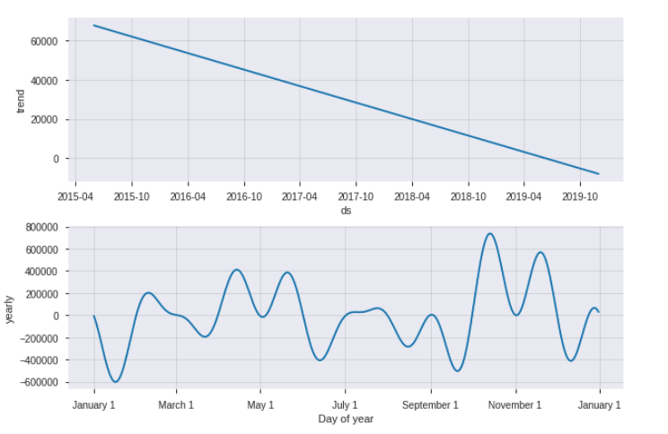
I would like to generate monthly seasonality insights with the results of prophet from my monthly data. @bletham has already explained in great way in the previous comments with help of plot_components method. However, graph isn't so clear to understand and keeping/extracting the information seems impossible. That's why, I tried to take average of yearly columns in forecast table to understand the monthly seasonality, but it doesn't match with graph comes from plot_components model.

plot_component result

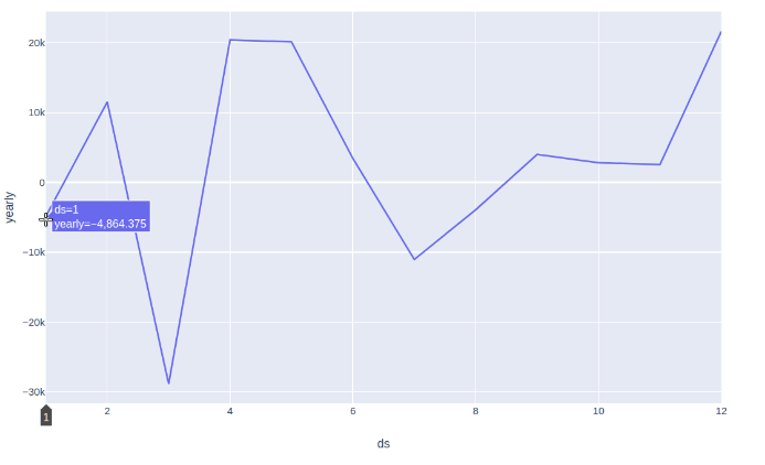
manually created yearly result

• Is it still okay to give such information looking at second plot(ignoring the first one)? If it is not how can I get monthly seasonality information?
  "The number of -4.8K for January indicates that every January, -4.8K of the y(sales) is attributed to the fact that it is January. It means that being on January has a -4.8K effect on y(sales). (ds indicates the month)"

Thanks!!
Used case in below.

import pandas as pd
from fbprophet import Prophet
from fbprophet import plot
from pandas import Timestamp
import plotly.express as px

#Import data
dict = {'ds': [Timestamp('2015-06-01 00:00:00'),
  Timestamp('2015-07-01 00:00:00'),
  Timestamp('2015-08-01 00:00:00'),
  Timestamp('2015-09-01 00:00:00'),
  Timestamp('2015-10-01 00:00:00'),
  Timestamp('2015-11-01 00:00:00'),
  Timestamp('2015-12-01 00:00:00'),
  Timestamp('2016-01-01 00:00:00'),
  Timestamp('2016-02-01 00:00:00'),
  Timestamp('2016-03-01 00:00:00'),
  Timestamp('2016-04-01 00:00:00'),
  Timestamp('2016-05-01 00:00:00'),
  Timestamp('2016-06-01 00:00:00'),
  Timestamp('2016-07-01 00:00:00'),
  Timestamp('2016-08-01 00:00:00'),
  Timestamp('2016-09-01 00:00:00'),
  Timestamp('2016-10-01 00:00:00'),
  Timestamp('2016-11-01 00:00:00'),
  Timestamp('2016-12-01 00:00:00'),
  Timestamp('2017-01-01 00:00:00'),
  Timestamp('2017-02-01 00:00:00'),
  Timestamp('2017-03-01 00:00:00'),
  Timestamp('2017-04-01 00:00:00'),
  Timestamp('2017-05-01 00:00:00'),
  Timestamp('2017-06-01 00:00:00'),
  Timestamp('2017-07-01 00:00:00'),
  Timestamp('2017-08-01 00:00:00'),
  Timestamp('2017-09-01 00:00:00'),
  Timestamp('2017-10-01 00:00:00'),
  Timestamp('2017-11-01 00:00:00'),
  Timestamp('2017-12-01 00:00:00'),
  Timestamp('2018-01-01 00:00:00'),
  Timestamp('2018-02-01 00:00:00'),
  Timestamp('2018-03-01 00:00:00'),
  Timestamp('2018-04-01 00:00:00'),
  Timestamp('2018-05-01 00:00:00'),
  Timestamp('2018-06-01 00:00:00'),
  Timestamp('2018-07-01 00:00:00'),
  Timestamp('2018-08-01 00:00:00'),
  Timestamp('2018-09-01 00:00:00'),
  Timestamp('2018-10-01 00:00:00'),
  Timestamp('2018-11-01 00:00:00'),
  Timestamp('2018-12-01 00:00:00'),
  Timestamp('2019-01-01 00:00:00'),
  Timestamp('2019-02-01 00:00:00'),
  Timestamp('2019-03-01 00:00:00'),
  Timestamp('2019-04-01 00:00:00'),
  Timestamp('2019-05-01 00:00:00'),
  Timestamp('2019-06-01 00:00:00')],
 'y': [115368.716,
  53018.181,
  85211.22799999997,
  66031.138,
  33773.054,
  70598.0412,
  101016.8463,
  83210.6998,
  47467.138600000006,
  41461.794,
  89416.93609999999,
  41566.638,
  27250.230199999998,
  27237.804600000003,
  37200.081,
  43102.188799999996,
  64780.19,
  41915.49,
  32714.890000000003,
  37011.09,
  59143.56999999999,
  62233.98,
  52959.590000000004,
  3713.1500000000005,
  16335.490000000002,
  21662.84,
  6408.6,
  19462.260000000002,
  42437.76,
  14617.729999999998,
  14375.820000000002,
  19561.749999999996,
  28358.140000000003,
  17308.660000000003,
  13878.01,
  33600.52,
  22124.399999999998,
  15859.25,
  11915.940000000002,
  38236.16999999999,
  15747.609999999999,
  22887.01,
  48057.68000000001,
  8980.57,
  2723.31,
  11638.0,
  26332.56,
  2182.45,
  8955.259999999998]}
df = pd.DataFrame.from_dict(dict)
df.columns = ['ds', 'y']

#Train default additive model
m = Prophet()
m.fit(df)

#Create 6 months prediction dataframe
future = m.make_future_dataframe(periods=6, freq ='M')
#Forecasting
forecast = m.predict(future)

#Plot results
m.plot_components(forecast).show()

#Yearly seasonality graphs
a = forecast.groupby([forecast['ds'].dt.month])['yearly'].mean().reset_index()
fig = px.line(a, x="ds", y="yearly")
fig.show()

[bletham]

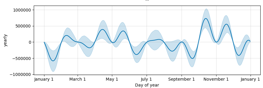
The issue here with the seasonality fit is that with monthly data, the yearly seasonality for dates other than the first day of each month are not really identifiable, and the model can do pretty funky things in those periods. This is described in the documentation here: https://facebook.github.io/prophet/docs/non-daily_data.html#monthly-data

On this time series, if you do MCMC you can see that these big spikes are happening in areas with no data (mid-month) and can see the uncertainty there:

m = Prophet(mcmc_samples=500)

The manually created result is the right way to look at the yearly seasonality that is actually being used (that just on the first-of-month dates). With monthly data you'll probably also want to add some extra regularization, for instance

m = Prophet(seasonality_prior_scale=0.1)

will get the two plots looking a bit more similar.

As described in the documentation page above, the root of the difference is that yearly seasonality is being modeled in continuous time but data points are only given at a sparse, discrete set of points. A better way to model yearly seasonality for monthly data is probably to fit a binary regressor for which month it is. You can do this with by creating a binary indicator for each month and adding it as a regressor:

m = Prophet(yearly_seasonality=False)

months = ['jan', 'feb', 'mar', 'apr', 'may', 'jun', 'jul', 'aug', 'sep', 'oct', 'nov', 'dec']
for i, month in enumerate(months):
    df[month] = (df['ds'].dt.month == i + 1).values.astype('float')
    m.add_regressor(month)

Then the model will no longer try to extrapolate mid-month values and gives a reasonable seasonality effect:

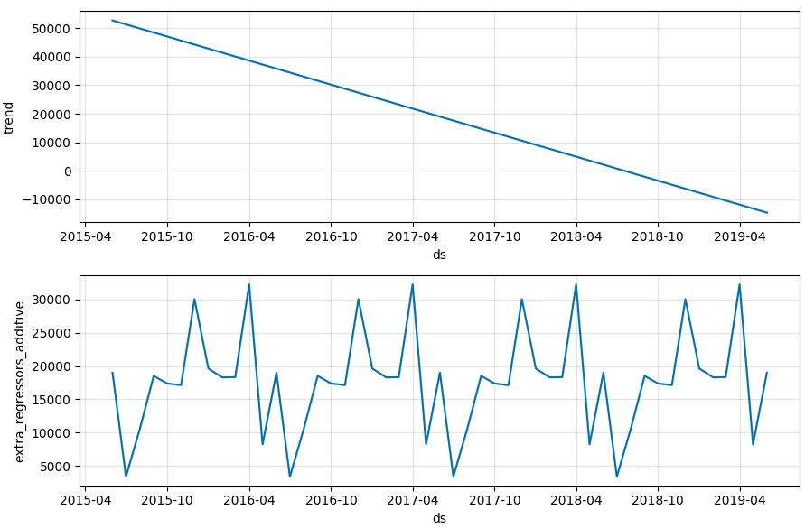
We should probably put this approach in the documentation actually.

[candalfigomoro]

@bletham
One problem I'm seeing with the binary indicator for months, is that I get a high coefficient not only for months with "real" periodic seasonalities, but I also get a high coefficient for months where there's a one-time spike in values (a one-time spike which is not repeated across years). I tried to change the prior scale for the binary regressors, but it affects the regressors coefficient both for "real periodic seasonalities" and one-time spikes. Is there a way to capture the "periodic seasonalities" (e.g. a spike consistently repeated every March) without the effect of one-time spikes which are not repeated across years?

The only thing that comes to mind is to remove one-time spikes/outliers before fitting Prophet, but it's not trivial (you also have to consider the trend etc.). Is there a better approach? Thanks.

[bletham]

Using a binary indicator for the month, basically what it will fit will be something like the average increase across years (since it is minimizing mean squared error). So if you do have a month with a spike, it will drag up the average.

I think the best thing to do in this case would be to also add a holiday for the one-time spike date. This would tell the model that there is something happening in addition to the yearly seasonality, and I'd expect it to use the holiday effect to capture the spike while yearly seasonality would capture only the repeated pattern.

[bletham]

The documentation update this was left open for has now been made.