Lightgbm: Interaction constraints

[mayer79]

Feature interaction

Monotonicity constraints is one way to make the black-box more intuitive and interpretable. For tree based models, using Interaction constraints is another highly interesting possibility: Passing a nested list like [[0, 1], [2]] specifies which features may be selected in the same tree branch, see explanations in https://github.com/dmlc/xgboost/issues/4075 in general and https://discuss.xgboost.ai/t/feature-interaction-constraint-overlap/506 for what happens if the sets overlap.

Quoting hcho3: "Let S the set of features used in all the ancestor nodes of the proposed split (plus itself). The proposed split is admitted whenever at least one set in the interaction constraint is a superset of S."

I think this would be a big step towards making boosted trees more interpretable and to e.g. being able to specify "additive" components as well as to reflect ethical constraints into a model.

[guolinke]

It seems is a very interesting feature, contribution is very welcomed.
And I will implement it when I have time and if no PR is proposed.

[mayer79]

That would be simply fantastic as my C++ skills are even worse than me speaking French. Still, you can test the implementation e.g. with Friedman's H statistic, a model agnostic approach to measure interaction strength. It is implemented in R packages iml and flashlight (mine):

library(xgboost)

n <- 1000
m <- 4

set.seed(1)
X <- matrix(rnorm(n * m), ncol = m, dimnames = list(NULL, paste0("X", 1:m)))
cols <- colnames(X)
y <- X[, 1] * X[, 2] * X[, 3] + X[, 4] + rnorm(n)

params <- list(
  learning_rate = 0.1,
  depth = 4, 
  objective = "reg:linear",
  #interaction_constraints = list(0, c(1, 2, 3)) # col index starts at 0
  interaction_constraints = list(0, 1, 2, 3) # col index starts at 0
)

train <- xgb.DMatrix(X, label = y)

fit <- xgb.train(params, train, nrounds = 50)


library(flashlight)
fl <- flashlight(model = fit, data = data.frame(y, X), y = "y", label = "xgb",
                 predict_fun = function(m, X) predict(m, data.matrix(X[, cols])))
plot(imp <- light_interaction(fl, v = cols, pairwise = FALSE))

The first parametrization gives

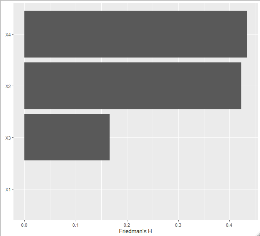
while the second one gives

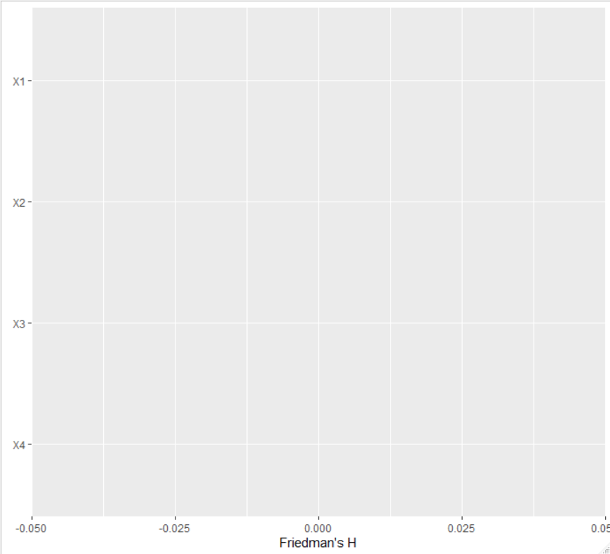
Setting pairwise = TRUE would show bars for each variable pair.

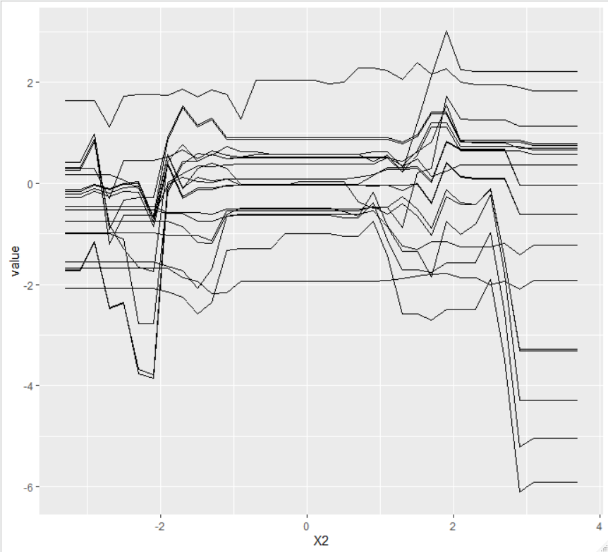
An even simpler approach is to look at ceteris paribus profiles (the heart of partial dependence plots). For variables without interactions, the curves must be parallel.

For the first parametrization of the interaction_constraints, we get for the first variable:

plot(light_ice(fl, v = "X1", seed = 1))

And for the second variable:

[StrikerRUS]

Implemented in #3126.