Lightgbm: Quantile regression in LightGBM

[mandeldm]

Currently LightGBM does not appear to support 'quantile' loss metric. (This is a feature that can be found in sklearn's Gradient Boosting Regression http://scikit-learn.org/stable/auto_examples/ensemble/plot_gradient_boosting_quantile.html - helpful if one wishes to construct margins of error / probability distribution for each prediction.)

Are there plans to include quantile regression in this product?

Thank you.

[mandeldm]

Adding a possible starting point:
https://www.bigdatarepublic.nl/regression-prediction-intervals-with-xgboost/ wherein Benoit Descamps provides an implementation of quantile_loss for xgboost (his code and results are near the bottom of the page).

His version of the loss function includes additional parameters which he calibrates using grid search. I don't feel qualified to say whether this implementation is completely correct or optimal.

[ClimbsRocks]

This would be awesome, and for me, illustrates one of the biggest gaps between using ML academically, and using it in production environments.

Every time we ship a new ML predictor, one of the first questions people ask is "Can you tell me which of these predictions you're confident in, and which ones have more uncertainty, so we can take different actions accordingly?". Sklearn's implementation of this is the best answer I've yet found to that question. But it's _so_ slow.

If we could have that same functionality, but at lightgbm speeds and accuracies, we'd be pretty darn happy :) At that point, we'd probably make prediction intervals the default behavior in auto.ml, because this functionality is so frequently useful.

[guolinke]

I think the first problem is to define a metric for quantile loss. Any suggestions?

[mandeldm]

I would suggest the same metric (sometimes called the "check" function, probably for the checkmark shape of its graph) that QuantileLossFunction uses in https://github.com/scikit-learn/scikit-learn/blob/master/sklearn/ensemble/gradient_boosting.py

My intuition for it is that the mean absolute error is the loss function for the median = 50th percentile, and "tilting" the MAE graph to the right (for lower percentiles) or to the left (for higher) gives us the general quantile loss function. I also found this brief lecture video and this explanation helpful.

As I suggested in my earlier comment, the quantile regression gradient & hessian calculation method Benoit Descamps outlined in his post for xgboost is worth exploring here.

Thanks.

[guolinke]

@mandeldm thanks very much, they are very helpful.
@henry0312 What do you think the MAE by the 50-per quantile regression ?

[henry0312]

I haven't caught up the loss metric yet.
I'll try.

[chivee]

@guolinke , I think Benoit Descamps's implementation is quite logical, maybe we can implement it as an prototype?

[ClimbsRocks]

If you do, I'll try to test it on a couple of our datasets, and compare it to sklearn for consistency

[guolinke]

@ClimbsRocks you can test PR #1043, I think it is almost done.

[ClimbsRocks]

It appears to be working, (and is quite quick!), but I'm not sure that it's taking in user-inputted alpha values. I'm getting very similar results whether I pass in an alpha of .05 or .4. I'll look into this more over the weekend, there's a decent chance it's just a bug in my code.

I'm using the sklearn interface:

LGBMRegressor(alpha=0.95, boosting_type='gbdt', colsample_bytree=1.0,
       lambda_l2=0.001, learning_rate=0.15, max_bin=255, max_depth=-1,
       min_child_samples=20, min_child_weight=0.001, min_split_gain=0.0,
       n_estimators=2000, n_jobs=-1, num_leaves=8, objective='quantile',
       random_state=0, reg_alpha=0.0, reg_lambda=0.0, silent=True,
       subsample=1.0, subsample_for_bin=200000, subsample_freq=1)

For what it's worth, I'm doing this on just a small test dataset (Boston house prices), so maybe it just needs a larger sample to work properly.

Thanks for the quick progress on this!

[guolinke]

The PR is merged.
feel free to feedback.

[ClimbsRocks]

Sweet, thanks for building this quickly!

[mandeldm]

@guolinke Thank you for your hard work on this.
I tried to replicate the prediction intervals from http://scikit-learn.org/stable/auto_examples/ensemble/plot_gradient_boosting_quantile.html, but was unable to. Changing alpha from 0.95 to 0.05 does not appear to change the prediction. That seems consistent with what @ClimbsRocks observed earlier.

I took the code from the above sklearn GBR page and replaced the GBR estimator with LGBMRegressor everywhere (additions are bracketed with ## ADDED & ## END ADDED).

If anyone could let me know whether I'm doing something wrong here, I'd be grateful.

%matplotlib inline
import numpy as np
import matplotlib.pyplot as plt


## ADDED
import lightgbm as lgb
## END ADDED


from sklearn.ensemble import GradientBoostingRegressor

np.random.seed(1)


def f(x):
    """The function to predict."""
    return x * np.sin(x)

#----------------------------------------------------------------------
#  First the noiseless case
X = np.atleast_2d(np.random.uniform(0, 10.0, size=100)).T
X = X.astype(np.float32)

# Observations
y = f(X).ravel()

dy = 1.5 + 1.0 * np.random.random(y.shape)
noise = np.random.normal(0, dy)
y += noise
y = y.astype(np.float32)

# Mesh the input space for evaluations of the real function, the prediction and
# its MSE
xx = np.atleast_2d(np.linspace(0, 10, 1000)).T
xx = xx.astype(np.float32)

alpha = 0.95

# clf = GradientBoostingRegressor(loss='quantile', alpha=alpha,
#                                 n_estimators=250, max_depth=3,
#                                 learning_rate=.1, min_samples_leaf=9,
#                                 min_samples_split=9)

# clf.fit(X, y)


## ADDED
clf = lgb.LGBMRegressor(objective='quantile',
                        alpha=alpha,
                        num_leaves=31,
                        learning_rate=0.05,
                        n_estimators=100)
clf.fit(X, y,
        eval_set=[(X, y)],
        eval_metric='quantile',
        early_stopping_rounds=5)
## END ADDED


# Make the prediction on the meshed x-axis
y_upper = clf.predict(xx)

# clf.set_params(alpha=1.0 - alpha)
# clf.fit(X, y)


## ADDED
clf.set_params(alpha=1.0 - alpha)
clf.fit(X, y,
        eval_set=[(X, y)],
        eval_metric='quantile',
        early_stopping_rounds=5)
## END ADDED


# Make the prediction on the meshed x-axis
y_lower = clf.predict(xx)

# clf.set_params(loss='ls')
# clf.fit(X, y)


## ADDED
clf.set_params(objective='regression', eval_metric='l2')
clf.fit(X, y,
        eval_set=[(X, y)],
        eval_metric='l2',
        early_stopping_rounds=5)
## END ADDED


# Make the prediction on the meshed x-axis
y_pred = clf.predict(xx)

# Plot the function, the prediction and the 90% confidence interval based on
# the MSE
fig = plt.figure()
plt.plot(xx, f(xx), 'g:', label=u'$f(x) = x\,\sin(x)$')
plt.plot(X, y, 'b.', markersize=10, label=u'Observations')
plt.plot(xx, y_pred, 'r-', label=u'Prediction')
plt.plot(xx, y_upper, 'k-')
plt.plot(xx, y_lower, 'k-')
plt.fill(np.concatenate([xx, xx[::-1]]),
         np.concatenate([y_upper, y_lower[::-1]]),
         alpha=.5, fc='b', ec='None', label='90% prediction interval')
plt.xlabel('$x$')
plt.ylabel('$f(x)$')
plt.ylim(-10, 20)
plt.legend(loc='upper left')
plt.show()

[ClimbsRocks]

Thanks for the reproducible code snippet, @mandeldm ! That's infinitely more helpful than my report above :)

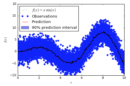
To help orient anyone who's new to this chart and code snippet (it's not one of sklearn's finest or most readable pieces of code), here's what the chart "should" look like, using the sklearn version:

And here's what the lgbm version looks like:

Obviously, the sklearn version has a band around the predictions, while the lgbm version has a band of 0 width that shows up as a black line. Interestingly, the band doesn't appear to be consistently higher or lower than the predictions, it just appears to wander through them somewhat at random.

Looking at two orders of magnitude more samples is also interesting:

Here's the sklearn version:

And here's the lgbm version:

[guolinke]

@mandeldm @ClimbsRocks
it seems sklearn interface has some bugs, I tested it by using native lightgbm interface:
code:

import numpy as np
import matplotlib.pyplot as plt
import lightgbm as lgb
from sklearn.ensemble import GradientBoostingRegressor

np.random.seed(1)


def f(x):
    """The function to predict."""
    return x * np.sin(x)

#----------------------------------------------------------------------
#  First the noiseless case
X = np.atleast_2d(np.random.uniform(0, 10.0, size=100)).T
X = X.astype(np.float32)

# Observations
y = f(X).ravel()

dy = 1.5 + 1.0 * np.random.random(y.shape)
noise = np.random.normal(0, dy)
y += noise
y = y.astype(np.float32)

# Mesh the input space for evaluations of the real function, the prediction and
# its MSE
xx = np.atleast_2d(np.linspace(0, 10, 1000)).T
xx = xx.astype(np.float32)

alpha = 0.95

params = {"objective":"quantile", 
"alpha": alpha,
"max_depth": 8, 
"num_leaves": 50,
"learning_rate": 0.1,
"verbose": -1, 
"metric": "quantile",
"min_data": 9}

lgb_train = lgb.Dataset(X, y)

clf = lgb.train(params, lgb_train, valid_sets=lgb_train, num_boost_round=250)

# Make the prediction on the meshed x-axis
y_upper = clf.predict(xx)

params["alpha"] = 1.0 - alpha
clf = lgb.train(params, lgb_train, valid_sets=lgb_train, num_boost_round=250)

# Make the prediction on the meshed x-axis
y_lower = clf.predict(xx)

params["objective"] = "regression"
clf = lgb.train(params, lgb_train, num_boost_round=250)

# Make the prediction on the meshed x-axis
y_pred = clf.predict(xx)


# Plot the function, the prediction and the 90% confidence interval based on
# the MSE
fig = plt.figure()
plt.plot(xx, f(xx), 'g:', label=u'$f(x) = x\,\sin(x)$')
plt.plot(X, y, 'b.', markersize=10, label=u'Observations')
plt.plot(xx, y_pred, 'r-', label=u'Prediction')
plt.plot(xx, y_upper, 'k-')
plt.plot(xx, y_lower, 'k-')
plt.fill(np.concatenate([xx, xx[::-1]]),
         np.concatenate([y_upper, y_lower[::-1]]),
         alpha=.5, fc='b', ec='None', label='95% prediction interval')
plt.xlabel('$x$')
plt.ylabel('$f(x)$')
plt.ylim(-10, 20)
plt.legend(loc='upper left')
plt.show()

result: