Lightgbm: Maybe a bug about Hessian matrix of regression_l1 objective function

[WXFMAV]

Maybe a bug about Hessian matrix of regression_l1 objective function

There may be a bug in Hessian matrix of regression_l1 objective function.

It was strange and unreasonable in function ApproximateHessianWithGaussian that the gaussian variance is set as
const double c = std::max((std::fabs(y) + std::fabs(t)) * eta, 1.0e-10);

The proper code maybe as
const double c = std::max((std::fabs(y-t)) * eta, 1.0e-10);

Though I am not very sure if this is a bug, my program fails in weighted sampling as is reported in issue https://github.com/Microsoft/LightGBM/issues/939

reference:
The Code in File: https://github.com/Microsoft/LightGBM/blob/master/src/objective/regression_objective.hpp
between line 98 and line 123

  void GetGradients(const double* score, score_t* gradients,
                    score_t* hessians) const override {
    if (weights_ == nullptr) {
      #pragma omp parallel for schedule(static)
      for (data_size_t i = 0; i < num_data_; ++i) {
        const double diff = score[i] - label_[i];
        if (diff >= 0.0f) {
          gradients[i] = 1.0f;
        } else {
          gradients[i] = -1.0f;
        }
        hessians[i] = static_cast<score_t>(Common::ApproximateHessianWithGaussian(score[i], label_[i], gradients[i], eta_));
      }
    } else {
      #pragma omp parallel for schedule(static)
      for (data_size_t i = 0; i < num_data_; ++i) {
        const double diff = score[i] - label_[i];
        if (diff >= 0.0f) {
          gradients[i] = weights_[i];
        } else {
          gradients[i] = -weights_[i];
        }
        hessians[i] = static_cast<score_t>(Common::ApproximateHessianWithGaussian(score[i], label_[i], gradients[i], eta_, weights_[i]));
      }
    }
  }

And the code in File:
https://github.com/Microsoft/LightGBM/blob/87fa8b542e0027e03027197ba07aab2812d6755d/include/LightGBM/utils/common.h
between line 486 and line 495

inline static double ApproximateHessianWithGaussian(const double y, const double t, const double g,
                                                    const double eta, const double w=1.0f) {
  const double diff = y - t;
  const double pi = 4.0 * std::atan(1.0);
  const double x = std::fabs(diff);
  const double a = 2.0 * std::fabs(g) * w;  // difference of two first derivatives, (zero to inf) and (zero to -inf).
  const double b = 0.0;
  const double c = std::max((std::fabs(y) + std::fabs(t)) * eta, 1.0e-10);
  return w * std::exp(-(x - b) * (x - b) / (2.0 * c * c)) * a / (c * std::sqrt(2 * pi));
}

[Laurae2]

ping @henry0312

[Tony-Y]

@WXFMAV Please see Representations of the delta function.
This code employs the heat kernel for the delta function approximation. c in this code may be a small positive number.

[Tony-Y]

@guolinke BTW, why does b exist?

Why not as the following?

return w * std::exp(-x * x / (2.0 * c * c)) * a / (c * std::sqrt(2 * pi));

[henry0312]

I'm sorry I don't have time to check the issue and remember the reason.

[henry0312]

Oh, I just remembered!

BTW, why does b exist?

b is the position of the center of the peak, so I wanted to clarify the shape of gaussian function.

cf. https://en.wikipedia.org/wiki/Gaussian_function

[henry0312]

When I have free time, I'll check this issue, sorry.

[henry0312]

cf. https://github.com/Microsoft/LightGBM/pull/178#issuecomment-271280902

[Tony-Y]

@henry0312 I have some questions.

1. Gradients are the Heaviside step function, but are not approximated as a smooth function in contrast of hessians that are the Dirac delta function. Can this inconsistency be disregarded?

2. The small number c depends on both the variable y (score) and the constant t (label). Is it reasonable that c depends on y?

3. Can the global number c be determined from a statistical value of whole labels?

[Tony-Y]

If c must depend on y, I think it should be a function of x=|y-t| in order to preserve the symmetry.

For example,

const double diff = y - t;
const double x = std::fabs(diff);
const double c = std::max(x + std::fabs(t)) * eta, 1.0e-10);

[henry0312]

I have checked this issue and your questions and organised my answers (in Japanese), but it will take some time to write them in English (because of my poor English...).

[Tony-Y]

I found the objective function that has hessians in any form. A brief description is shown below.

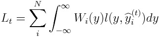
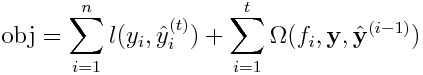
We introduce the label weighting function W_i(y), and define the objective function L_t as a weighted mean of loss function l(y,y^).

The Taylor expansion ofL_t is given as:

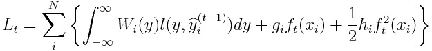
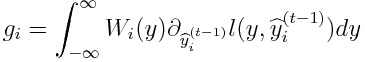
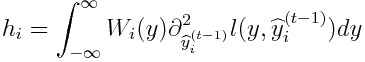
If l(y,y^) = |y - y^|, we obtain:


Hence, we can have hessians in any form.

I hope users and developers have any idea.

[Tony-Y]

I take some notes on approximations to the delta or step function.

1. Logistic Approximation to Step Function
   The logistic function f(x) is a smooth approximation to the step function.
   https://en.m.wikipedia.org/wiki/Heaviside_step_function#Analytic_approximations
   The derivative of f(x) is df/dx = f(x)f(1-x) = 𝞓(x), and an approximation to the delta function.
   https://en.m.wikipedia.org/wiki/Logistic_function#Derivative
   The weighting function can be defined as:
   W_i(y) = 𝞓((y - y_i)/T)
   where T is the temperature parameter.
   In physics, f(x) is known as the Fermi–Dirac distribution.

2. Methfessel-Paxton Approximation to Step Function
   http://www.hector.ac.uk/cse/distributedcse/reports/conquest/conquest/node6.html
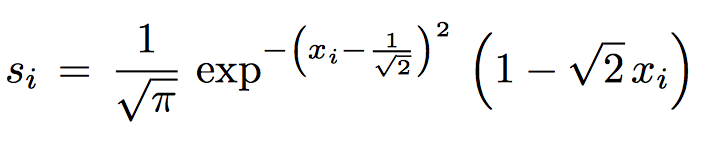
   The N-th order approximation to the delta function:
   
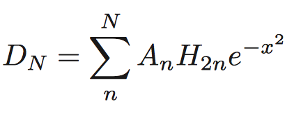
   where A_n are suitable coefficients, and H_n are Hermite polynomials.
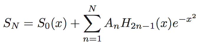
   The N-th order approximation to the step function:
   
   

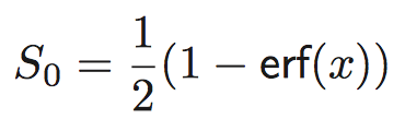
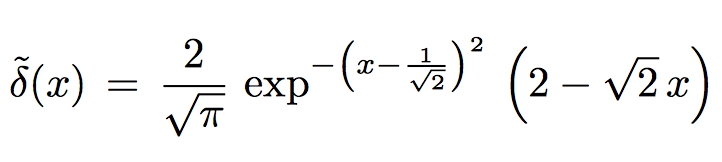
3. Marzari-Vanderbilt Approximation to Delta Function
   https://arxiv.org/pdf/cond-mat/9903147.pdf
   The approximation to the delta function:
   
   The approximation to the step function:
   

[Tony-Y]

Please see:
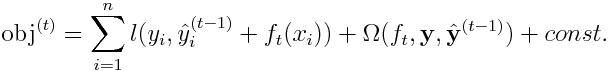
https://xgboost.readthedocs.io/en/latest/model.html

Suppose that each label y_i is not exactly equal to the prediction y_i^ for all time.
If the loss function is the mean absolute error, gradients are +1 or -1, and hessians are all zero.
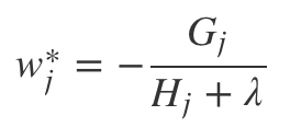
If the L2 regularization parameter 𝝺 is non-zero, we obtain:
w_j* = - G_j/𝝺
obj* = -1/2 ∑ (G_j)^2/𝝺 + 𝛄T
On condition that the first assumption is reasonably valid, the algorithm probably works well.

[Tony-Y]

@henry0312 The above investigation would suggest that the approximate hessian you introduced is like a variable 𝝺. However, I can't get the exact mathematical expression yet.

What do you think about my suggestion?

[Tony-Y]

I conclude that Henry0312's approach is a special case of the method based on the following objective:

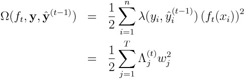
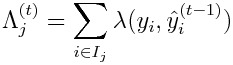
where

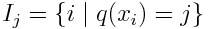
When the loss function is the absolute error, we have to make it reasonably valid that each label y_i is not exactly equal to the prediction y_i^ for all time. In order to do so, the L2 weight function 𝛌 should be defined as a positive monatomic decreasing function of the absolute value of the difference between the label and the prediction:

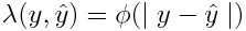
For example:

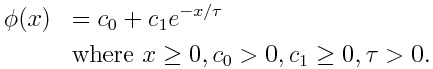
The L2 weight function 𝜆 resembles a hessian when the loss function is the absolute error. However, 𝜆 does not come from the approximation to the delta function.

@henry0312 If you agree with the above, please review and test your code on the basis of the objective with variable L2 weights.

[Tony-Y]

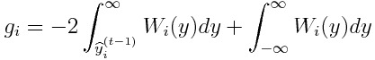
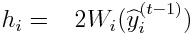
If we would like to remove the assumption that y_i ≠ y^_i when the loss function is the absolute error, we must ensure that
w_j* = 0
where i ∈ I_j and y_i = y^_i, because the sum of hessians H_j is infinity.

(This figure was taken from https://xgboost.readthedocs.io/en/latest/model.html)

[Tony-Y]

@guolinke I found two necessary conditions for using the absolute error as the loss function:

1. Use of the L2 regularization
2. Each label is not exactly equal to the corresponding prediction for all time

Condition 1 is subject to the objective function, but Condition 2 is subject to splitting a leaf.
In numerical implementation, when splitting a leaf at step t, the following inequality must be satisfied:

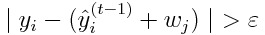
where 𝛆 > (machine epsilon).

Can you code this algorithm in the related source codes?

[henry0312]

Please wait until next week.
I'm too busy to work for LightGBM.

2017年10月18日(水) 20:54 Tony-Y [e-mail]:

@guolinke https://github.com/guolinke I found two necessary conditions
for using the absolute error as the loss function:

1. Use of the L2 regularization
2. Each label is not exactly equal to the corresponding prediction for
   all time

Condition 1 is subject to the objective function, but Condition 2 is
subject to splitting a leaf.
In numerical implementation, when splitting a leaf at step t, the
following inequality must be satisfied:
[image: condition_2]
https://user-images.githubusercontent.com/11532812/31715974-fc58d4de-b440-11e7-8e8e-3081eeba676f.png
where 𝛆 > (machine epsilon).

Can you code this algorithm in the related source codes?

—
You are receiving this because you were mentioned.

Reply to this email directly, view it on GitHub
https://github.com/Microsoft/LightGBM/issues/979#issuecomment-337566337,
or mute the thread
https://github.com/notifications/unsubscribe-auth/AAadGuPDlSE47ut4f1EwxbDBocijyh0jks5stebcgaJpZM4PyYm7
.

[gugatr0n1c]

Couple months ago I run some tests on this. Using gradients from {-1, 1} never worked good enough for me.
I got best results for L1 task with this:

def myObj(preds, train_data):
labels = train_data.get_label()
grad = np.sign(preds - labels) * np.abs(preds - labels)**0.5
hess = [1.] * len(preds)
return grad, hess

Because gradients only with elements from {-1, 1} are "too stupid" for this algorithm.
The part: "np.abs(preds - labels)0.5" helping algorithm to converge but it is not so aggressive as for L2. You can also run smaller exponent like: np.abs(preds - labels)0.25

But this is only practical observation.

[Tony-Y]

@guolinke BTW, do you really need the objective with the L1 loss? Actually, I don't need it.

[guolinke]

@Tony-Y I always use the solution like the @gugatr0n1c provided.
And using some label conversions in regression is equivalent to changing objective function.

[gugatr0n1c]

Btw when I run some stacking (multiple models with different hyper parameters) I always add some model with objective like above. Even for L2 (MSE) task. The reason is: this form of gradients converge to different solution and brings new variability from data. It is like "free lunch". Almost in all datasets are some outliers pushing L2 norm to not so optimal solution (known drawback of L2).
But this is little bit offtopic.

[Tony-Y]

@guolinke Thank you for your reply. I had focused on mathematical aspect too much. I leave from this thread.

@gugatr0n1c Thank you for letting me know your use case.

[henry0312]

I'll reply tonigt.

EDIT (1:48 (JST)): I just came back home, but I'm too tired to reply.

[Laurae2]

@henry0312 Any news?

[guolinke]

please try the one solution in #1199