jupyter-book 🚀 - syntax and structure of TOC file

+1 to file and +1 to pages.

For the options about collapsing etc, that's actually a carryover from jupyter book. We are gonna be limited by yaml syntax but could try playing around with different structure.

choldgraf on 8 Mar 2020

check out the latest changes merged in https://github.com/ExecutableBookProject/cli/pull/27 ... wdyt?

choldgraf on 8 Mar 2020

A quick update on this - I asked around on Twitter (in a totally unscientific way) and this was the result:

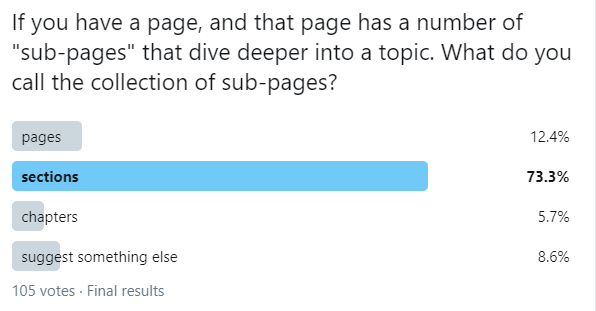
Should that influence our thinking about "pages" vs "sections"? "pages" was second, though a distant second.

re: your sections syntax etc, we could try for something like:

- file: my/page
  sections:
    - not_numbered: true
    - expand_sections: true
    - file: page1
    - file: page2

Though in that case, we are conflating section-wide metadata with pages within the section in the same "sections" list...

choldgraf on 26 Mar 2020

Yes, this should influence our thinking :-). Nice idea to run a poll, and I agree that my pages suggestion was suboptimal!

But let's consider this: Since our mental model is a book, where do we see chapters fitting into the structure above, when we convert to LaTeX? Even if we get this clear in our heads, what about our users?

In bookdown the structure is really simple. It's just

file: preface
file: intro
file: some_definitions
file: main_results
file: conclusion

The rules are:

Each file corresponds to a chapter once the book is generated
If you want sections/subsections use (# Section A, ## Subsection B, etc.) inside each of these files.

To me this is super clear and corresponds to the right mental model --- writing a book.

Each of these files listed in the TOC can be associated with one ipynb file.

The next most important use-case after writing a book is writing a lecture series, and again this simple vertical structure works perfectly for that.

file: about_this_course
file: lecture_1
file: lecture_2
file: lecture_3
file: conclusion

Finally, in this space that we're operating in, we have exactly one highly successful data point and that's bookdown. I suspect they're so successful because the basic structure is so simple (and the output is so good).

jstac on 26 Mar 2020

Thanks @jstac for starting this thread.

I think simplicity is the right aim here -- while the tradeoff is less ability to control at the section level -- the main case for books is usually a global style that applies to all within chapter sections such as:

numbering chapters and sections
local table of contents for each Chapter

My main concern with flat structure is how to control Parts (which we use on QuantEcon, essentially support for nested table of contents) and Front matter.

I tend to think the top level toc should have the ability to configure book elements that are chapter level and above such as Parts, book title, book author and other front matter.

The downside is less control for the static site generator use case.

In my mind it might be nice to consider domains for the toc file where the language lines up with the context. We could have toc.book, toc.site, toc.article that provide interfaces to the different domain use. This grant would of course focus on toc.book.

mmcky on 27 Mar 2020

It looks like bookdown puts front matter in index.Rmd file

https://github.com/rstudio/bookdown/blob/master/inst/examples/index.Rmd

witch special markup to control numbering at the end of the titles

mmcky on 27 Mar 2020

Yes, my proposal (follow bookdown) doesn't allow for "parts", as in "Part 1", "Part II", etc., which can be used to group chapters.

We could start without and then think about adding them in phase 2 of deployment? Bookdown seems to be popular despite lacking them.

jstac on 27 Mar 2020

Another pattern here is GitBook, which uses a summary file to define the book structure:

https://docs.gitbook.com/integrations/github/content-configuration#summary

e.g.:

# Summary

## Use headings to create page groups like this one

* [First page's title](page1/README.md)    
    * [Some child page](page1/page1-1.md)    
    * [Some other child page](part1/page1-2.md)

* [Second page's title](page2/README.md)    
    * [Some child page](page2/page2-1.md)    
    * [Some other child page](part2/page2-2.md)    

## A second-page group

* [Yet another page](another-page.md)

This is the closest inspiration for how Jupyter Book defines its book structure though it makes some things more explicit (like "heading: my heading" etc).

My mental model is that there is one page per file, and so chapters are naturally collections of pages (ie, collections of files). So to me, if I wanted to organize my jupyter-book as a "traditional" book (ie, with chapters each of which has multiple pages), then I'd use strict "top-level pages all have multiple pages as sections" structure.

choldgraf on 27 Mar 2020

Can I suggest that we keep our terminology matched up to the hierarchy

parts -> chapters -> sections -> subsections

rather than talking about, say, pages, as I did before, or child pages, as in this example? That will help us focus on providing users with the clearest structure for writing a book (as opposed to producing an arbitrary website, which is definitely not a service that we're offering).

In that terminology, what I'm saying is, let's let each file correspond to one chapter, with the level 1 heading as the title of the chapter, level 2 headings delineating sections, level 3 headings denoting subsections, etc.

That's a very simple model, it's what bookdown does, and it's extremely successful, so, in my view, it should be the default, and we would need some reason to deviate from it.

chapters are naturally collections of pages (ie, collections of files)

OK, to express this in my book-centric terminology above, what you're saying is that each md file, which we can think of as in one-to-one correspondence with an ipynb file / notebook, is going to map to a section, right? That is, the level below chapter.

So, for an unsophisticated user who comes to us with a collection of ipynb files, under your proposal, we say to them that "each of your notebooks will be a section in your book, and you can group those sections together into chapters by using syntax XYZ in the TOC". Correct?

That seems reasonable too.

jstac on 27 Mar 2020

OK, to express this in my book-centric terminology above, what you're saying is that each md file, which we can think of as in one-to-one correspondence with an ipynb file / notebook, is going to map to a section, right? That is, the level below chapter.

Not quite - I'd say that each .md or .ipynb file is a page. Pages can be lots of things. Some books have chapters, some have sub-chapters, and others are just a flat collection of pages. A page can have sections and sub-sections, which are delimited by #H1 and #H2 etc.

So to me, a page is always a single file (.md or .ipynb). A chapter is a collection of pages with an overarching theme. A book is either a collection of chapters or a collection of pages.

I think that my default approach is to try and not be opinionated about the terminology we force people to use. It's why I have shied away from using "book-like" words like "chapters" in favor of more generic words like "sections". It's really hard to know what kind of mental model people will be coming with - if we're creating something like the inferential thinking textbook, or QuantEcon, then strong book-like words make sense. But I can also say that most of the Jupyter Book books out there are closer to flat collections of pages. E.g., to randomly pick one, this HelioML book is closer to a flat list of analyses

choldgraf on 27 Mar 2020

my default approach is to try and not be opinionated about the terminology we force people to use.

Mine is to be opinionated :-). I think people want guidance and simple rules when they try something new.

Not quite - I'd say that each .md or .ipynb file is a page.

That's a mental model for building a website, not a book. You have that in your head because you're a strong web developer, as well as a scientist :-).

But what does a "page" map to when you run it through LaTeX? Not a page of the resulting PDF, right? So the "page" terminology is confusing, unless we're going to say that the LaTeX version is a second class citizen.

Let's put ourselves in the position of an average scientist with a folder containing 10 ipynb files on a sequence of topics. She's never built a website before. She just wants to turn her files into a book as easily as possible.

In bookdown, all the TOC does is it allows you to tell the compiler which order these files should be presented in. The result is a PDF book with 10 chapters.

If she does the same thing with our tools, she also gets a website with 10 pages. Every one of them is also downloadable as an ipynb, ready to execute.

That's a super simple model that's very easy to get started with. Can't we start with that and then add fanciness if and when it's requested?

Your HelioML book example is, in essence, just a flat collection of ipynb files that would fit this model well.

jstac on 27 Mar 2020

But what does a "page" map to when you run it through LaTeX? Not a page of the resulting PDF, right? So the "page" terminology is confusing, unless we're going to say that the LaTeX version is a second class citizen.

In my case I'm defining "page" at the authoring process, not at the output process. To me, when I'm writing in an ipynb file, or in a markdown file, that's a page, regardless of whatever the end build product will be. There might be lots of different kinds of outputs, but the inputs will be consistent, so I'm trying to keep my mental model of the book structure defined at the input file level, rather than the output file.

I agree with your point about "guidance and simple rules". To me, saying "each markdown file is a page in the book, pages can also have collections of sub-pages underneath them, which together define a section" with a TOC like this:

- file: intro.md
  section:
    - file: a.md
    - file: b.md
      section:
        - file: c.md

feels like the simplest way of doing things. I think it has these benefits:

You can quickly get a birds-eye view of the structure of the book just by looking at this file (as opposed to just having a flat list of files, which themselves may have one or multiple sub-sections within them, but that you wouldn't be able to tell unless you actually opened the file
The TOC defined in the YAML file looks like the TOC that you'd show in any kind of output
You only need to know one word to create a book: "file". Additionally if they use the word "section" then they can now have a nested TOC hierarchy. That's it.
This maps exactly onto the model that Sphinx uses ("one input file per page"), and since we're using Sphinx under the hood, this simplifies the parsing process.

That's a super simple model that's very easy to get started with. Can't we start with that and then add fanciness if and when it's requested?

I'm not sure what is incompatible with our already-existing model? This just seems like:

- file: ntbka
- file: ntbkb
- file: ntbkc
- file: ntbkd
...

and that's it. Or am I missing something here?

choldgraf on 27 Mar 2020

@choldgraf are you saying that your structure is a superset of that proposed by @jstac? Can you specify a simple listing of chapters as files?

mmcky on 27 Mar 2020

It would be helpful if you guys gave a small toc.yml file that would define a book structure, it is hard for me to imagine what you have in mind.

What I'm saying is that an author only needs to know two words: "file" and "section". Any file can have a section underneath it. Sections are made up of one or more files. If authors want to think of collections of files, or individuals files, as chapters, or sections, or parts, that's fine, but users don't need to use a different word for each one in their table of contents file.

I'll give a few examples (I'll choose file names based on how I imagine the author to be conceptualizing these pages and their relation to the book).

If I wanted to define chapters, I could do either:

- file: chapter1.md
- file: chapter2.md

or I could do

- file: chapter1_intro.md
  section:
  - file: chapter1_page1.md
  - file: chapter1_page2.md
- file: chapter2_intro.md
  section:
  - file: chapter2_page1.md
  - file: chapter2_page2.md

if I wanted to add a "sub-chapter" then I'd do:

- file: chapter1_intro.md
  section:
  - file: chapter1_page1.md
  - file: chapter1_page2.md
- file: chapter2_intro.md
  section:
  - file: chapter2_page1.md
  - file: chapter2_page2.md
    section:
      - file: chapter1_page2_subpage1.md

It would be up to the author to decide however they want to organize their book - the vocabulary and building blocks available to them are simple and flexible enough that it could accommodate whatever they like. To that point, they also don't even need the concept of chapters. It could also be:

- file: page1.md
- file: page2.md

choldgraf on 27 Mar 2020

It would be up to the author to decide however they want to organize their book

Nooooooooo.

flexible enough that it could accommodate whatever they like.

Nooooooo. We should not offer them that. We'll totally confuse them.

file: chapter1_page1.md

But this does not correspond to a page in the PDF, so it's confusing? Don't you agree?

Why do you wish to be so cruel to your would-be users? :grin:

What I'm saying is, let's target the gazillion and one users out there that (a) have a bunch of ipynb files lying around and (b) know perfectly well what a book is --- and want to build one from their ipynb files.

If the hypothetical user comes to us with 10 ipynb files and says "hey, I want to turn these into a book", then we should say, so there's zero ambiguity, "sure bro, it breaks down like this: each of your ipynb files corresponds to one chapter in your book -- which is also one web page."

Zero confusion results.

I don't mind if we substitute the word "section" for "chapter" above. I just think we need to tell them what part of a book each of their ipynb files is.

jstac on 27 Mar 2020

Nooooooo. We should not offer them that. We'll totally confuse them.

FWIW (and I recognize this is not a rigorous datapoint) but anecdotally there are like 500 books that have been built w/ jupyter book (which has a similar kind of TOC structure to it), and nobody has ever brought up the TOC nomenclature as a confusion point. This is also similar to the TOC structure that GitBook uses, and as they are a growing company I assume they have put much more UI/UX researchers on that question than we will ever be able to...

But this does not correspond to a page in the PDF, so it's confusing? Don't you agree?

But again, to me the "page" is the source file, not whatever is in the output. But I agree that the word "page" is perhaps overloaded and means too many things that depend on context. Maybe that's not a good word to use.

each of your ipynb files corresponds to one chapter in your book

following my perspective from above - that the page is the source file - to me this sentence sounds like you are saying "each chapter of your book is always one page", which feels weird to me.

Let me sleep on this, I should be heading to bed. I'll try and play around with the word "chapter" or "section" to refer to a single ipynb or md file and see if I can get past the awkwardness, maybe it's just a mental hump to get over.

choldgraf on 27 Mar 2020

though again, it would be helpful if you'd give a concrete example. e.g., in the ideal "table of contents" structure that you'd like to see, how would I define a left sidebar like this:

and a right within-page (or section or chapter or whatever) TOC?

choldgraf on 27 Mar 2020

Thinking about this a bit more - what if we followed @jstac's suggestion and stop calling files "pages". That way we aren't potentially confusing the author. Instead, we follow John's hierarchy of:

chapters -> sections -> subsections

Chapters are generally seen as collections of sections.
Sections can have one or more subsections in them
The toc.yml file can be populated at a top level either with Chapters or sections.

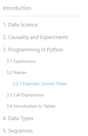
So the above image would be something like

- chapter: pathtointro.md
  title: Data Science
  sections:
    - section: pathtofile.md
    - section: pathtofile.md
      subsections:
        - section: pathtootherfile.md

In this case, jupyter book would behave in a more "book-like" way. Maybe Chapters would automatically be numbered, maybe there are other "chapter-specific" things you'd want to configure or do?

However, it would also be fine for users to only define sections in their toc.yml file:

- section: pathtointro.md
  title: Data Science
  subsections:
    - section: pathtofile.md
    - section: pathtofile.md
      subsections:
        - section: pathtootherfile.md

In that case, the CLI would be less-opinionated about what it should do with those sections. It would behave similarly to the same structure but with chapters though.

The only hard constraint here is that the key "chapter" and "section" (and maybe some other book-structure primitives) cannot both be present in the same entry.

Questions

Does this reasonably remove the confusion around the word "pages"?
Are there particular things that you can imagine wanting to do with a "chapter" item, as opposed to a "section" item? E.g. "chapters are automatically numbered"
- Here I am thinking about, for example, the fact that Sphinx has multiple "reference-style" roles. It has the {any} role as a catch-all for a generic reference. But is also has more specific {ref}, {doc}, etc roles if you know something is more specific. Maybe we are talking about the same kind of thing at the book level (maybe section:chapter::{any}:{ref}?).
- Then you could even imagine having other kinds of top-level items that were treated differently, like "preface" or "epilogue" or "introduction"

choldgraf on 27 Mar 2020

Would also love to hear any thoughts from @gregcaporaso on this one!

choldgraf on 27 Mar 2020

Thanks for your thoughts @choldgraf. Let me try to be more specific.

My concern is that we are currently overfitting to the HTML output case. Starting from the premise that HTML and LaTeX/PDF are equally important, how should we set up the TOC structure?

Note that LaTeX has the following numbered "sections" that can be cross referenced.

part > chapter > section > subsection > subsubsection

We have to decide how all of our headings are going to map to these objects when we translate to LaTeX, as well as think of how they look as nested HTML pages.

If we adopt the flat structure I'm proposing, your JB concrete example looks like this:

introduction.md
data_science.md
causality_and_experiments.md
python_programming.md
data_types.md
sequences.md

Inside python_programming.md you see

# Programming in Python

## Expressions

### Example: Growth Rates

## Names

## Call Expressions

## Introduction to Tables

That creates the TOC in the png you provided. When mapped to LaTeX, each level 1 header maps to a chapter, each level 2 header maps to a section, each level 3 header maps to a subsection, etc.
When mapped to HTML, each file is one web page.

It's limited but there's no ambiguity and it's easy to understand.

Now, let me ask you a question: Suppose you have, in your TOC structure, the following

- file: file_a.md
  section:
  - file: file_b.md
  - file: file_c.md
- file: file_d.md
  section:
  - file: file_e.md
  - file: file_f.md
    section:
      - file: file_g.md
      section:
        - file: file_h.md

Suppose that, in each one of these files, you have markdown headers from level 1 to level 4 (i.e, from # to ####). How are we going to map these to the LaTeX delineation given above?

And, additional challenge, how can this be explained to a would-be user, how wants to have an idea of what their book will look like before they start, in 1 sentence of simple English?

This issue is why I'm emphasizing that we're not creating arbitrary websites. GitBook, an example you allude to, doesn't map to LaTeX when it generates PDFs -- at least as far as I can tell.

jstac on 27 Mar 2020

Thanks for the clarification - some thoughts

My concern is that we are currently overfitting to the HTML output case. Starting from the premise that HTML and LaTeX/PDF are equally important, how should we set up the TOC structure?

that makes sense and I agree with the goal - I am trying to also avoid the opposite. Latex is notorious for confusing people, so I don't want to pull confusing UX pieces from Latex just because we are more familiar with it. To use your average data scientist user, in my experience the average data scientist has much more experience with a structure like gitbook summary files than with latex-style delineation of parts/chapters/sections/subsections/etc.

To me, the flat hierarchy is harder to understand, because it doesn't actually tell me about the structure of the book beyond the first level. I'll know how many top-level sections there are, but that's it. In order to understand the structure of the book I'd have to open each file, see how many sections or sub-sections are inside, etc. The Table of Contents in a rendered output (be it a PDF or an HTML page) would not look like a flat list, and this would confuse me.

re: how to map a TOC like that onto PDF via Latex...I'd start by doing whatever Sphinx does. It already allows for arbitrary nested pages, and also already allows for PDF output via latex, no? Perhaps Sphinx puts a hard constraint on things like how many sub-pages you can have etc? I think we could say something like "if you want XXX expected behavior out of your PDF outputs, then you can have a maximum of 2 nested sections".

And, additional challenge, how can this be explained to a would-be user, how wants to have an idea of what their book will look like before they start, in 1 sentence of simple English?

(cheating and using two sentences)
I'd say 'Each input file is a section of content, and these can be grouped together as sub-sections if you wish. In a website, subsections will be revealed when a user visits its introduction page; in a PDF, sections and subsections are mapped onto Latex "parts" and "chapters"'.

choldgraf on 27 Mar 2020

Another consideration is in reading content and then sending people to the source files. E.g., in Jupyter Book a key interaction mechanism is to have Binder links that send you to notebooks, or to have "download source" buttons so that people can start running through content themselves. If you can only have one input file per top-level section, then many people who currently have a nested structure would need to have one gigantic ipynb file for each chapter.

For example, this chapter of the data 8 textbook is made up of 6 notebooks that operate in a modular fashion. In a flat TOC structure, this would need to be a single, gigantic, Jupyter Notebook with multiple sections within it, no?

choldgraf on 27 Mar 2020

Why don't we impose a hard-constraint on the nesting that's available in the TOC? Basically say "the TOC can't have more than two nested levels". Then, assuming a Latex-style structure:

part > chapter > section > subsection > subsubsection

First level in TOC -> part
Second level in TOC -> chapter
Third level in TOC -> section
Headers in a page: subsection & subsubsection

Then you could have the mapping onto Latex, we just don't need to call these things "parts, chapters, etc" in the _toc.yml file itself.

choldgraf on 27 Mar 2020

I like to hear you say the the word "constraints" and I'm glad we're trying to specify this map but I don't think that constraint will be sufficient.

Let's go back to my file_a -- file_h example. But let's eliminate file_h because it's nested to the third level. This agrees with your proposal:

- file: file_a.md
  section:
  - file: file_b.md
  - file: file_c.md
- file: file_d.md
  section:
  - file: file_e.md
  - file: file_f.md
    section:
      - file: file_g.md

Here's my question again, referring to that example:

Suppose that, in each one of these files, you have markdown headers from level 1 to level 4 (i.e, from # to ####). How are we going to map these to the LaTeX delineation given above?

The LaTeX delineation is part > chapter > section > subsection > subsubsection

What will you map a level 4 header to if it's in file_a?

What will you map a level 4 header to if it's in file_g?

jstac on 27 Mar 2020

I'd say "markdown files can have at most 2 levels in them (at least as far as PDF output goes), corresponding to ## and ### (assuming that # is reserved for the title) and mapping onto subsection and subsubsection in the PDF output. For PDF outputs, any header that is higher than ### will be mapped on to ###/\subsubsection

Assuming that it was header level ### instead of ####, it would map to something like:

\part file_a
      \subsubsection `###`

  \chapter file_b
  \chapter file_c
\part file_d
  \chapter file_f
    \section file_g
      \subsubsection `###`

I would describe a guiding principle behind this as: "it's better to have more input files that are more modular, rather than fewer input files that have lots of mixed content and topics in them." I think that this also follows best-practices in analysis with Jupyter Notebooks.

Or put another way, if we have 6 "layers" to work with in a book:

part > chapter > section > subsection > subsubsection

You're suggesting that

* part <-- a page is here
* chapter <-- these are controlled by # headers
* section 
* subsection 
* subsubsection

I'm suggesting that

* part <-- these are controlled by the TOC file
* chapter 
* section <-- a page is here 
* subsection <-- these are controlled by # headers
* subsubsection

also, just another note that it will be easier to start uncovering the challenges associated with this if folks started making progress with a Latex / PDF exporter. These discrepancies are partially arriving now because I've been the only one working on the CLI, and I don't have the latex perspective that y'all do. Is there a plan to make progress on this?

choldgraf on 27 Mar 2020

I think we're converging. But in your outcome

\part file_a
      \subsubsection `###`

  \chapter file_b
  \chapter file_c
\part file_d
  \chapter file_f
    \section file_g
      \subsubsection `###`

the compilation would fail because you can't have a subsubsection under a part.

"markdown files can have at most 2 levels in them (at least as far as PDF output goes), corresponding to ## and ### (assuming that # is reserved for the title) and mapping onto subsection and subsubsection in the PDF output.

I don't think that will work, for the reason given above. The mapping would need to be sensitive to the level of nesting. If it's a chapter level file, then ## needs to be section, if it's a section level file, then ## needs to be subsection, so we go down by one step at each time.

In the bookdown model, none of these issues arise.

Regarding the LaTeX writer, this depends on @mmcky and @AakashGfude, and I've slowed them down by asking them to split the QE Python lectures into three subprojects: https://python.quantecon.org/

I hope, however, that this will make it easier to port material when the time comes.

jstac on 27 Mar 2020

So how does sphinx do things then? They've had sphinx documentation -> PDF via latex for years now. We're using the same fundamental structure that Sphinx uses in its sites...

Looking at the binderhub docs and the PDF generated by readthedocs, it looks like:

A top-level toctree group maps onto a chapter in Latex (https://binderhub.readthedocs.io/en/latest/index.html#zero-to-binderhub). The "caption" of the toctree becomes the first text of that chapter.
each item in the toctree maps onto a section: https://binderhub.readthedocs.io/en/latest/zero-to-binderhub/index.html#zero-to-binderhub
All within-page headers that are greater than ## are flattened to ##.

So that would assume something like:

- introduction: path/to/intropage
  chapters:
    - chapter: Chapter title
      caption: The introduction to chapter 1
      sections:
      - section: path/to/page1
      - section: path/to/page2
    - chapter: Chapter 2 title
      caption: The introduction to chapter 2
      sections:
        - section: path/to/page3
        - section: path/to/page4

maybe you could simplify that to

- introduction: path/to/intro
  chapters:
    - chapter: path/to/chapter1_intro
      sections:
      - section: path/to/page1
      - section: path/to/page2
    - chapter: path/to/chapter2_intro
      sections:
        - section: path/to/page3
        - section: path/to/page4

I frame it in this way because ultimately, we are going to need to translate the "table of contents" file into some combination of toctree objects on actual pages in Sphinx.

choldgraf on 27 Mar 2020

Perhaps @mmcky could step in here. Their toc structure is a bit different to the yaml approach. It works well for our QE material.

jstac on 27 Mar 2020

hey @choldgraf happy to link up to discuss this in more details in real time sometime soon. The main difficulty with high degree of flexible construction of the toc is when mapping to LaTeX. Keeping to your examples above we would need to setup a tex file that contains the frontmatter and toc and then append all sections into a single tex file that represents a chapter.

For sphinxcontrib-jupyter -- our current approach is to build a index file from the top level index rst file. The latex files are then compiled per rst file (mapping an rst file to a chapter which is often done when writing latex books). The index file includes chapter titles and a file include to the chapter tex file.

One alternative approach might be to build a single book tex file and append all content into the same file in the order specified by the toc. My concern here though is if you are writing a file such as path/to/page2 it will be natural to start at the top with a single # for the title rather than using the appropriate title depth based on the context of the book. This is much easier to keep track of if writing in chapter chunks / file as the book title is a special case and all other titles are localised (as @jstac points out above)

re: Titles I also think we should try and infer as much as possible from the source files.

Here is the main tex file produced by sphinxcontrib-jupyter for a book which makes it pretty easy to read.

\cleardoublepage\part{Introduction to Python}
\chapter{About Python}\input{about_py.tex}
\chapter{Setting up Your Python Environment}\input{getting_started.tex}
\chapter{An Introductory Example}\input{python_by_example.tex}
\chapter{Functions}\input{functions.tex}
\chapter{Python Essentials}\input{python_essentials.tex}
\chapter{OOP I: Introduction to Object Oriented Programming}\input{oop_intro.tex}
\chapter{OOP II: Building Classes}\input{python_oop.tex}

mmcky on 28 Mar 2020

Hey @mmcky - thanks for the input! I have been spending the morning trying to get Latex set up on my computer so that I can test out the Sphinx PDF building functionality. As you can probably guess, this has been a two-hour rabbit hole of trying to install things and I still don't have it working, but I hope to test it out soon. Gahhhh latex!

as an aside - I am really worried about how much effort it takes to get latex up and running. In my experience the large majority of users across the sciences - particularly younger ones - have never used latex before. I am a pretty proficient coder and familiar with Ubuntu, and have also installed latex probably a half dozen times before. However it has taken me almost 2 hours of debugging to get this set up and I'm still not getting a built PDF. We need to make sure the documentation is excellent for this part of things...

It sounds like the sphinxcontrib-jupyter approach is quite similar to what Sphinx itself does by default. My intuition is that we should be trying to mimic the Sphinx PDF builder as much as possible, ideally we'd be using the default PDF builder, and we'd upstream improvements that need to be made to it, perhaps with our own customizations for look and feel, and for nodes that are jupyter-book-specific. I think that follows in line with our principles and constraints regarding using pre-existing tools and patterns wherever possible

If you run make latexpdf then it generates a master tex file that looks like this.

The headers in the "index page" become chapters
Each toctree item in the "index page" becomes a section
Each toctree item in a section page become a subsection
Any H2-level headers in a subsection become sub-subsections
Any higher headers become \paragraph{} elements

For example, here is the myst-nb docs built with the latex builder:

%% Generated by Sphinx.
\def\sphinxdocclass{report}
\documentclass[letterpaper,10pt,english]{sphinxmanual}
\ifdefined\pdfpxdimen
   \let\sphinxpxdimen\pdfpxdimen\else\newdimen\sphinxpxdimen
\fi \sphinxpxdimen=.75bp\relax

\PassOptionsToPackage{warn}{textcomp}
\usepackage[utf8]{inputenc}
\ifdefined\DeclareUnicodeCharacter
% support both utf8 and utf8x syntaxes
  \ifdefined\DeclareUnicodeCharacterAsOptional
    \def\sphinxDUC#1{\DeclareUnicodeCharacter{"#1}}
  \else
    \let\sphinxDUC\DeclareUnicodeCharacter
  \fi
  \sphinxDUC{00A0}{\nobreakspace}
  \sphinxDUC{2500}{\sphinxunichar{2500}}
  \sphinxDUC{2502}{\sphinxunichar{2502}}
  \sphinxDUC{2514}{\sphinxunichar{2514}}
  \sphinxDUC{251C}{\sphinxunichar{251C}}
  \sphinxDUC{2572}{\textbackslash}
\fi
\usepackage{cmap}
\usepackage[T1]{fontenc}
\usepackage{amsmath,amssymb,amstext}
\usepackage{babel}



\usepackage{times}
\expandafter\ifx\csname T@LGR\endcsname\relax
\else
% LGR was declared as font encoding
  \substitutefont{LGR}{\rmdefault}{cmr}
  \substitutefont{LGR}{\sfdefault}{cmss}
  \substitutefont{LGR}{\ttdefault}{cmtt}
\fi
\expandafter\ifx\csname T@X2\endcsname\relax
  \expandafter\ifx\csname T@T2A\endcsname\relax
  \else
  % T2A was declared as font encoding
    \substitutefont{T2A}{\rmdefault}{cmr}
    \substitutefont{T2A}{\sfdefault}{cmss}
    \substitutefont{T2A}{\ttdefault}{cmtt}
  \fi
\else
% X2 was declared as font encoding
  \substitutefont{X2}{\rmdefault}{cmr}
  \substitutefont{X2}{\sfdefault}{cmss}
  \substitutefont{X2}{\ttdefault}{cmtt}
\fi


\usepackage[Bjarne]{fncychap}
\usepackage{sphinx}

\fvset{fontsize=\small}
\usepackage{geometry}


% Include hyperref last.
\usepackage{hyperref}
% Fix anchor placement for figures with captions.
\usepackage{hypcap}% it must be loaded after hyperref.
% Set up styles of URL: it should be placed after hyperref.
\urlstyle{same}

\usepackage{sphinxmessages}




\title{MyST\sphinxhyphen{}NB}
\date{Mar 28, 2020}
\release{}
\author{Executable Book Project}
\newcommand{\sphinxlogo}{\vbox{}}
\renewcommand{\releasename}{}
\makeindex
\begin{document}

\pagestyle{empty}
\sphinxmaketitle
\pagestyle{plain}
\sphinxtableofcontents
\pagestyle{normal}
\phantomsection\label{\detokenize{index::doc}}


A collection of tools for working with Jupyter Notebooks in Sphinx, using the
Markedly Structured Text markdown language.

The primary tool this package provides is a Sphinx parser for \sphinxcode{\sphinxupquote{ipynb}} files.
This allows you to directly convert Jupyter Notebooks into Sphinx documents.
It relies heavily on the \sphinxhref{https://github.com/ExecutableBookProject/myst\_parser}{\sphinxcode{\sphinxupquote{MyST}} parser}.

A secondary tool is the ‘glue’ functionality, outlined in the {\hyperref[\detokenize{use/glue:glue}]{\sphinxcrossref{\DUrole{std,std-ref}{Inserting variables with glue}}}} section,
which allows outputs of notebook code cells to be accessed and displayed anywhere within the documentation (even from different files).

\begin{sphinxadmonition}{warning}{Warning:}
This project is in an alpha state. It may evolve rapidly and/or make breaking changes!
Comments, requests, or bugreports are welcome and recommended! Please
\sphinxhref{https://github.com/ExecutableBookProject/myst-nb/issues}{open an issue here}
\end{sphinxadmonition}


\chapter{Installation}
\label{\detokenize{index:installation}}
To install \sphinxcode{\sphinxupquote{myst\sphinxhyphen{}nb}}, do the following:
\begin{itemize}
\item {} 
Install \sphinxcode{\sphinxupquote{myst\sphinxhyphen{}nb}} with the following command:

\begin{sphinxVerbatim}[commandchars=\\\{\}]
pip install myst\PYGZhy{}nb
\end{sphinxVerbatim}

Or for package development:

\begin{sphinxVerbatim}[commandchars=\\\{\}]
git clone https://github.com/ExecutableBookProject/MyST\PYGZhy{}NB
\PYG{n+nb}{cd} MyST\PYGZhy{}NB
git checkout master
pip install \PYGZhy{}e .\PYG{o}{[}code\PYGZus{}style,testing,rtd\PYG{o}{]}
\end{sphinxVerbatim}

\item {} 
Enable the \sphinxcode{\sphinxupquote{myst\_nb}} extension in your Sphinx repository’s extensions:

\begin{sphinxVerbatim}[commandchars=\\\{\}]
\PYG{n}{extensions} \PYG{o}{=} \PYG{p}{[}
    \PYG{o}{.}\PYG{o}{.}\PYG{o}{.}\PYG{p}{,}
    \PYG{l+s+s2}{\PYGZdq{}}\PYG{l+s+s2}{myst\PYGZus{}nb}\PYG{l+s+s2}{\PYGZdq{}}
\PYG{p}{]}
\end{sphinxVerbatim}

\begin{sphinxadmonition}{note}{Note:}
If you’d like to use MyST to parse markdown files as well, then you can enable it by
adding \sphinxcode{\sphinxupquote{myst\_parser}} to your list of extensions as well.
\end{sphinxadmonition}

\item {} 
Write Jupyter Notebooks with your built documentation, and remember to include them
in your \sphinxcode{\sphinxupquote{toctree}}, and that’s it!

\end{itemize}


\chapter{How the Jupyter Notebook parser works}
\label{\detokenize{index:how-the-jupyter-notebook-parser-works}}
MyST\sphinxhyphen{}NB is built on top of the MyST markdown parser. This is a flavor of markdown
designed to work with the Sphinx ecosystem. It is a combination of CommonMark markdown,
with a few extra syntax pieces added for use in Sphinx (for example, roles and
directives).

\begin{sphinxadmonition}{note}{Note:}
For more about MyST markdown, see
\sphinxhref{https://myst-parser.readthedocs.io/en/latest/}{the MyST markdown documentation}
\end{sphinxadmonition}

MyST\sphinxhyphen{}NB will do the following:
\begin{itemize}
\item {} 
Check for any pages in your documentation folder that end in \sphinxcode{\sphinxupquote{.ipynb}}. For each one:

\item {} 
Loop through the notebook’s cells, converting cell contents into the Sphinx AST.
\begin{itemize}
\item {} 
If it finds executable code cells, include their outputs in\sphinxhyphen{}line with the code.

\item {} 
If it finds markdown cells, use the MyST parser to convert them into Sphinx.

\end{itemize}

\end{itemize}

Eventually, it will also provide support for writing pure\sphinxhyphen{}markdown versions of notebooks
that can be executed and read into Sphinx.


\chapter{Use and configure}
\label{\detokenize{index:use-and-configure}}
For information on using and configuring MyST\sphinxhyphen{}NB, as well as some examples of notebook
outputs, see the pages below:


\section{Use and customize}
\label{\detokenize{use/index:use-and-customize}}\label{\detokenize{use/index::doc}}
A collection of example pages to see how notebook content is rendered
in Sphinx with MyST\sphinxhyphen{}NB.


\subsection{An example Jupyter Notebook}
\label{\detokenize{use/basic:an-example-jupyter-notebook}}\label{\detokenize{use/basic::doc}}
This notebook is a demonstration of directly\sphinxhyphen{}parsing Jupyter Notebooks into
Sphinx using the MyST parser.


\subsubsection{Markdown}
\label{\detokenize{use/basic:markdown}}
As you can see, markdown is parsed as expected. Embedding images should work as expected.
For example, here’s the MyST\sphinxhyphen{}nb logo:

\sphinxincludegraphics{{logo}.png}

because MyST\sphinxhyphen{}NB is using the MyST\sphinxhyphen{}markdown parser, you can include rich markdown with Sphinx
in your notebook.%
\begin{footnote}[1]\sphinxAtStartFootnote
Even footnotes!
%
\end{footnote} For example, here’s a note block:

\begin{sphinxadmonition}{note}{Note:}
Wow, a note! It was generated with this code:

\begin{sphinxVerbatim}[commandchars=\\\{\}]
```\PYGZob{}note\PYGZcb{}
Wow, a note!

\end{sphinxVerbatim}
\end{sphinxadmonition}

subsubsection{Code cells and outputs}
\label{\detokenize{use/basic:code-cells-and-outputs}}
You can run cells, and the cell outputs will be captured and inserted into
the resulting Sphinx site.

\paragraph{\sphinxstyleliteralintitle{\sphinxupquote{__repr__}} and HTML outputs}
\label{\detokenize{use/basic:repr-and-html-outputs}}
For example, here’s some simple Python:

\begin{sphinxVerbatim}[commandchars=\{}]
\PYG{k+kn}{import} \PYG{n+nn}{matplotlib}\PYG{n+nn}{.}\PYG{n+nn}{pyplot} \PYG{k}{as} \PYG{n+nn}{plt}
\PYG{k+kn}{import} \PYG{n+nn}{numpy} \PYG{k}{as} \PYG{n+nn}{np}
\PYG{n}{data} \PYG{o}{=} \PYG{n}{np}\PYG{o}{.}\PYG{n}{random}\PYG{o}{.}\PYG{n}{rand}\PYG{p}{(}\PYG{l+m+mi}{3}\PYG{p}{,} \PYG{l+m+mi}{100}\PYG{p}{)} \PYG{o}{*} \PYG{l+m+mi}{100}
\PYG{n}{data}\PYG{p}{[}\PYG{p}{:}\PYG{p}{,} \PYG{p}{:}\PYG{l+m+mi}{10}\PYG{p}{]}
\end{sphinxVerbatim}

This will also work with HTML outputs

\begin{sphinxVerbatim}[commandchars=\{}]
\PYG{k+kn}{import} \PYG{n+nn}{pandas} \PYG{k}{as} \PYG{n+nn}{pd}
\PYG{n}{df} \PYG{o}{=} \PYG{n}{pd}\PYG{o}{.}\PYG{n}{DataFrame}\PYG{p}{(}\PYG{n}{data}\PYG{o}{.}\PYG{n}{T}\PYG{p}{,} \PYG{n}{columns}\PYG{o}{=}\PYG{p}{[}\PYG{l+s+s1}{\PYGZsq{}}\PYG{l+s+s1}{a}\PYG{l+s+s1}{\PYGZsq{}}\PYG{p}{,} \PYG{l+s+s1}{\PYGZsq{}}\PYG{l+s+s1}{b}\PYG{l+s+s1}{\PYGZsq{}}\PYG{p}{,} \PYG{l+s+s1}{\PYGZsq{}}\PYG{l+s+s1}{c}\PYG{l+s+s1}{\PYGZsq{}}\PYG{p}{]}\PYG{p}{)}
\PYG{n}{df}\PYG{o}{.}\PYG{n}{head}\PYG{p}{(}\PYG{p}{)}
\end{sphinxVerbatim}

This works for error messages as well:

\begin{sphinxVerbatim}[commandchars=\{}]
\PYG{n+nb}{print}\PYG{p}{(}\PYG{l+s+s2}{\PYGZdq{}}\PYG{l+s+s2}{This will be properly printed...}\PYG{l+s+s2}{\PYGZdq{}}\PYG{p}{)}
\PYG{n+nb}{print}\PYG{p}{(}\PYG{n}{thiswont}\PYG{p}{)}
\end{sphinxVerbatim}

\paragraph{Images}
\label{\detokenize{use/basic:images}}
Images that are generated from your code (e.g., with Matplotlib) will also
be embedded.

\begin{sphinxVerbatim}[commandchars=\{}]
\PYG{n}{fig}\PYG{p}{,} \PYG{n}{ax} \PYG{o}{=} \PYG{n}{plt}\PYG{o}{.}\PYG{n}{subplots}\PYG{p}{(}\PYG{p}{)}
\PYG{n}{ax}\PYG{o}{.}\PYG{n}{scatter}\PYG{p}{(}\PYG{o}{*}\PYG{n}{data}\PYG{p}{,} \PYG{n}{c}\PYG{o}{=}\PYG{n}{data}\PYG{p}{[}\PYG{l+m+mi}{2}\PYG{p}{]}\PYG{p}{)}
\end{sphinxVerbatim}

\bigskip\hrule\bigskip

subsection{Widgets and interactive outputs}
\label{\detokenize{use/interactive:widgets-and-interactive-outputs}}\label{\detokenize{use/interactive::doc}}
Jupyter Notebooks have support for many kinds of interactive outputs.
These should all be supported in MyST\sphinxhyphen{}NB by passing the output HTML through
automatically.

This page has a few common examples. First off, we’ll download a little bit of data
and show its structure:

\begin{sphinxVerbatim}[commandchars=\{}]
\PYG{k+kn}{import} \PYG{n+nn}{plotly}\PYG{n+nn}{.}\PYG{n+nn}{express} \PYG{k}{as} \PYG{n+nn}{px}
\PYG{n}{data} \PYG{o}{=} \PYG{n}{px}\PYG{o}{.}\PYG{n}{data}\PYG{o}{.}\PYG{n}{iris}\PYG{p}{(}\PYG{p}{)}
\PYG{n}{data}\PYG{o}{.}\PYG{n}{head}\PYG{p}{(}\PYG{p}{)}
\end{sphinxVerbatim}

subsection{Plotting libraries}
\label{\detokenize{use/interactive:plotting-libraries}}

subsubsection{Altair}
\label{\detokenize{use/interactive:altair}}
Interactive outputs will work under the assumption that the outputs they produce have
self\sphinxhyphen{}contained HTML that works without requiring any external dependencies to load.
See the \sphinxhref{https://altair-viz.github.io/getting_started/installation.html#installation}{\sphinxcode{\sphinxupquote{Altair}} installation instructions}
to get set up with Altair. Below is some example output.

\begin{sphinxVerbatim}[commandchars=\{}]
\PYG{k+kn}{import} \PYG{n+nn}{altair} \PYG{k}{as} \PYG{n+nn}{alt}
\PYG{n}{alt}\PYG{o}{.}\PYG{n}{Chart}\PYG{p}{(}\PYG{n}{data}\PYG{o}{=}\PYG{n}{data}\PYG{p}{)}\PYG{o}{.}\PYG{n}{mark\PYGZus{}point}\PYG{p}{(}\PYG{p}{)}\PYG{o}{.}\PYG{n}{encode}\PYG{p}{(}
\PYG{n}{x}\PYG{o}{=}\PYG{l+s+s2}{\PYGZdq{}}\PYG{l+s+s2}{sepal\PYGZus{}width}\PYG{l+s+s2}{\PYGZdq{}}\PYG{p}{,}
\PYG{n}{y}\PYG{o}{=}\PYG{l+s+s2}{\PYGZdq{}}\PYG{l+s+s2}{sepal\PYGZus{}length}\PYG{l+s+s2}{\PYGZdq{}}\PYG{p}{,}
\PYG{n}{color}\PYG{o}{=}\PYG{l+s+s2}{\PYGZdq{}}\PYG{l+s+s2}{species}\PYG{l+s+s2}{\PYGZdq{}}\PYG{p}{,}
\PYG{n}{size}\PYG{o}{=}\PYG{l+s+s1}{\PYGZsq{}}\PYG{l+s+s1}{sepal\PYGZus{}length}\PYG{l+s+s1}{\PYGZsq{}}
\PYG{p}{)}
\end{sphinxVerbatim}

subsubsection{Plotly}
\label{\detokenize{use/interactive:plotly}}
Plotly is another interactive plotting library that provides a high\sphinxhyphen{}level API for
visualization. See the \sphinxhref{https://plotly.com/python/getting-started/#jupyterlab-support-python-35}{Plotly JupyterLab documentation}
to get started with Plotly in the notebook.

\begin{sphinxadmonition}{note}{Note:}
Plotly uses renderers to output different kinds of information when you display a plot. Using the
\sphinxcode{\sphinxupquote{plotly_mimetype}} renderer as below will cause the HTML to have a static PNG. Experiment with
the renderer option to get the output you want.
\end{sphinxadmonition}

Below is some example output.

\begin{sphinxVerbatim}[commandchars=\{}]
\PYG{k+kn}{import} \PYG{n+nn}{plotly}\PYG{n+nn}{.}\PYG{n+nn}{io} \PYG{k}{as} \PYG{n+nn}{pio}
\PYG{k+kn}{import} \PYG{n+nn}{plotly}\PYG{n+nn}{.}\PYG{n+nn}{express} \PYG{k}{as} \PYG{n+nn}{px}
\PYG{k+kn}{import} \PYG{n+nn}{plotly}\PYG{n+nn}{.}\PYG{n+nn}{offline} \PYG{k}{as} \PYG{n+nn}{py}

\PYG{n}{pio}\PYG{o}{.}\PYG{n}{renderers}\PYG{o}{.}\PYG{n}{default} \PYG{o}{=} \PYG{l+s+s2}{\PYGZdq{}}\PYG{l+s+s2}{plotly\PYGZus{}mimetype}\PYG{l+s+s2}{\PYGZdq{}}

\PYG{n}{df} \PYG{o}{=} \PYG{n}{px}\PYG{o}{.}\PYG{n}{data}\PYG{o}{.}\PYG{n}{iris}\PYG{p}{(}\PYG{p}{)}
\PYG{n}{fig} \PYG{o}{=} \PYG{n}{px}\PYG{o}{.}\PYG{n}{scatter}\PYG{p}{(}\PYG{n}{df}\PYG{p}{,} \PYG{n}{x}\PYG{o}{=}\PYG{l+s+s2}{\PYGZdq{}}\PYG{l+s+s2}{sepal\PYGZus{}width}\PYG{l+s+s2}{\PYGZdq{}}\PYG{p}{,} \PYG{n}{y}\PYG{o}{=}\PYG{l+s+s2}{\PYGZdq{}}\PYG{l+s+s2}{sepal\PYGZus{}length}\PYG{l+s+s2}{\PYGZdq{}}\PYG{p}{,} \PYG{n}{color}\PYG{o}{=}\PYG{l+s+s2}{\PYGZdq{}}\PYG{l+s+s2}{species}\PYG{l+s+s2}{\PYGZdq{}}\PYG{p}{,} \PYG{n}{size}\PYG{o}{=}\PYG{l+s+s2}{\PYGZdq{}}\PYG{l+s+s2}{sepal\PYGZus{}length}\PYG{l+s+s2}{\PYGZdq{}}\PYG{p}{)}
\PYG{n}{fig}
\end{sphinxVerbatim}

subsubsection{Bokeh}
\label{\detokenize{use/interactive:bokeh}}
Bokeh provides several options for interactive visualizations, and is part of the PyViz ecosystem. See
\sphinxhref{https://docs.bokeh.org/en/latest/docs/user_guide/jupyter.html#userguide-jupyter}{the Bokeh with Jupyter documentation} to
get started.

Below is some example output.

\begin{sphinxVerbatim}[commandchars=\{}]
\PYG{k+kn}{from} \PYG{n+nn}{bokeh}\PYG{n+nn}{.}\PYG{n+nn}{plotting} \PYG{k+kn}{import} \PYG{n}{figure}\PYG{p}{,} \PYG{n}{show}\PYG{p}{,} \PYG{n}{output\PYGZus{}notebook}
\PYG{n}{output\PYGZus{}notebook}\PYG{p}{(}\PYG{p}{)}

\PYG{n}{p} \PYG{o}{=} \PYG{n}{figure}\PYG{p}{(}\PYG{p}{)}
\PYG{n}{p}\PYG{o}{.}\PYG{n}{circle}\PYG{p}{(}\PYG{n}{data}\PYG{p}{[}\PYG{l+s+s2}{\PYGZdq{}}\PYG{l+s+s2}{sepal\PYGZus{}width}\PYG{l+s+s2}{\PYGZdq{}}\PYG{p}{]}\PYG{p}{,} \PYG{n}{data}\PYG{p}{[}\PYG{l+s+s2}{\PYGZdq{}}\PYG{l+s+s2}{sepal\PYGZus{}length}\PYG{l+s+s2}{\PYGZdq{}}\PYG{p}{]}\PYG{p}{,} \PYG{n}{fill\PYGZus{}color}\PYG{o}{=}\PYG{n}{data}\PYG{p}{[}\PYG{l+s+s2}{\PYGZdq{}}\PYG{l+s+s2}{species}\PYG{l+s+s2}{\PYGZdq{}}\PYG{p}{]}\PYG{p}{,} \PYG{n}{size}\PYG{o}{=}\PYG{n}{data}\PYG{p}{[}\PYG{l+s+s2}{\PYGZdq{}}\PYG{l+s+s2}{sepal\PYGZus{}length}\PYG{l+s+s2}{\PYGZdq{}}\PYG{p}{]}\PYG{p}{)}
\PYG{n}{show}\PYG{p}{(}\PYG{n}{p}\PYG{p}{)}
\end{sphinxVerbatim}

subsection{ipywidgets}
\label{\detokenize{use/interactive:ipywidgets}}
You may also run code for Jupyter Widgets in your document, and the interactive HTML
outputs will embed themselves in your side. See \sphinxhref{https://ipywidgets.readthedocs.io/en/latest/user_install.html}{the ipywidgets documentation}
for how to get set up in your own environment.

Here are some simple widget elements rendered below.

\begin{sphinxVerbatim}[commandchars=\{}]
\PYG{k+kn}{import} \PYG{n+nn}{ipywidgets} \PYG{k}{as} \PYG{n+nn}{widgets}
\PYG{n}{widgets}\PYG{o}{.}\PYG{n}{IntSlider}\PYG{p}{(}
\PYG{n}{value}\PYG{o}{=}\PYG{l+m+mi}{7}\PYG{p}{,}
\PYG{n+nb}{min}\PYG{o}{=}\PYG{l+m+mi}{0}\PYG{p}{,}
\PYG{n+nb}{max}\PYG{o}{=}\PYG{l+m+mi}{10}\PYG{p}{,}
\PYG{n}{step}\PYG{o}{=}\PYG{l+m+mi}{1}\PYG{p}{,}
\PYG{n}{description}\PYG{o}{=}\PYG{l+s+s1}{\PYGZsq{}}\PYG{l+s+s1}{Test:}\PYG{l+s+s1}{\PYGZsq{}}\PYG{p}{,}
\PYG{n}{disabled}\PYG{o}{=}\PYG{k+kc}{False}\PYG{p}{,}
\PYG{n}{continuous\PYGZus{}update}\PYG{o}{=}\PYG{k+kc}{False}\PYG{p}{,}
\PYG{n}{orientation}\PYG{o}{=}\PYG{l+s+s1}{\PYGZsq{}}\PYG{l+s+s1}{horizontal}\PYG{l+s+s1}{\PYGZsq{}}\PYG{p}{,}
\PYG{n}{readout}\PYG{o}{=}\PYG{k+kc}{True}\PYG{p}{,}
\PYG{n}{readout\PYGZus{}format}\PYG{o}{=}\PYG{l+s+s1}{\PYGZsq{}}\PYG{l+s+s1}{d}\PYG{l+s+s1}{\PYGZsq{}}
\PYG{p}{)}
\end{sphinxVerbatim}

\begin{sphinxVerbatim}[commandchars=\{}]
\PYG{n}{tab\PYGZus{}contents} \PYG{o}{=} \PYG{p}{[}\PYG{l+s+s1}{\PYGZsq{}}\PYG{l+s+s1}{P0}\PYG{l+s+s1}{\PYGZsq{}}\PYG{p}{,} \PYG{l+s+s1}{\PYGZsq{}}\PYG{l+s+s1}{P1}\PYG{l+s+s1}{\PYGZsq{}}\PYG{p}{,} \PYG{l+s+s1}{\PYGZsq{}}\PYG{l+s+s1}{P2}\PYG{l+s+s1}{\PYGZsq{}}\PYG{p}{,} \PYG{l+s+s1}{\PYGZsq{}}\PYG{l+s+s1}{P3}\PYG{l+s+s1}{\PYGZsq{}}\PYG{p}{,} \PYG{l+s+s1}{\PYGZsq{}}\PYG{l+s+s1}{P4}\PYG{l+s+s1}{\PYGZsq{}}\PYG{p}{]}
\PYG{n}{children} \PYG{o}{=} \PYG{p}{[}\PYG{n}{widgets}\PYG{o}{.}\PYG{n}{Text}\PYG{p}{(}\PYG{n}{description}\PYG{o}{=}\PYG{n}{name}\PYG{p}{)} \PYG{k}{for} \PYG{n}{name} \PYG{o+ow}{in} \PYG{n}{tab\PYGZus{}contents}\PYG{p}{]}
\PYG{n}{tab} \PYG{o}{=} \PYG{n}{widgets}\PYG{o}{.}\PYG{n}{Tab}\PYG{p}{(}\PYG{p}{)}
\PYG{n}{tab}\PYG{o}{.}\PYG{n}{children} \PYG{o}{=} \PYG{n}{children}
\PYG{n}{tab}\PYG{o}{.}\PYG{n}{titles} \PYG{o}{=} \PYG{p}{[}\PYG{n+nb}{str}\PYG{p}{(}\PYG{n}{i}\PYG{p}{)} \PYG{k}{for} \PYG{n}{i} \PYG{o+ow}{in} \PYG{n+nb}{range}\PYG{p}{(}\PYG{n+nb}{len}\PYG{p}{(}\PYG{n}{children}\PYG{p}{)}\PYG{p}{)}\PYG{p}{]}
\PYG{n}{tab}
\end{sphinxVerbatim}

subsection{Hiding cell contents}
\label{\detokenize{use/hiding:hiding-cell-contents}}\label{\detokenize{use/hiding::doc}}
You can use Jupyter Notebook \sphinxstylestrong{cell tags} to control some of the behavior of
the rendered notebook. This uses the \sphinxhref{https://sphinx-togglebutton.readthedocs.io/en/latest/}{\sphinxstylestrong{\sphinxcode{\sphinxupquote{sphinx\sphinxhyphen{}togglebutton}}}}
package to add a little button that toggles the visibility of content.

subsection{Hiding code cells}
\label{\detokenize{use/hiding:hiding-code-cells}}\label{\detokenize{use/hiding:use-hiding-code}}
You can \sphinxstylestrong{cell tags} to control the content hidden with code cells.
Add the following tags to a cell’s metadata to control
what to hide in code cells:
\begin{itemize}
\item {}
\sphinxstylestrong{\sphinxcode{\sphinxupquote{hide_input}}} tag to hide the cell inputs

\item {}
\sphinxstylestrong{\sphinxcode{\sphinxupquote{hide_output}}} to hide the cell outputs

\item {}
\sphinxstylestrong{\sphinxcode{\sphinxupquote{hide_cell}}} to hide the entire cell

\end{itemize}

For example, we’ll show cells with each below.

Here is a cell with a \sphinxcode{\sphinxupquote{hide_input}} tag. Click the “toggle” button to the
right to show it.

\begin{sphinxVerbatim}[commandchars=\{}]
\PYG{c+c1}{\PYGZsh{} This cell has a hide\PYGZus{}input tag}
\PYG{n}{fig}\PYG{p}{,} \PYG{n}{ax} \PYG{o}{=} \PYG{n}{plt}\PYG{o}{.}\PYG{n}{subplots}\PYG{p}{(}\PYG{p}{)}
\PYG{n}{ax}\PYG{o}{.}\PYG{n}{scatter}\PYG{p}{(}\PYG{o}{*}\PYG{n}{data}\PYG{p}{,} \PYG{n}{c}\PYG{o}{=}\PYG{n}{data}\PYG{p}{[}\PYG{l+m+mi}{0}\PYG{p}{]}\PYG{p}{,} \PYG{n}{s}\PYG{o}{=}\PYG{n}{data}\PYG{p}{[}\PYG{l+m+mi}{0}\PYG{p}{]}\PYG{p}{)}
\end{sphinxVerbatim}

Here’s a cell with a \sphinxcode{\sphinxupquote{hide_output}} tag:

\begin{sphinxVerbatim}[commandchars=\{}]
\PYG{c+c1}{\PYGZsh{} This cell has a hide\PYGZus{}output tag}
\PYG{n}{fig}\PYG{p}{,} \PYG{n}{ax} \PYG{o}{=} \PYG{n}{plt}\PYG{o}{.}\PYG{n}{subplots}\PYG{p}{(}\PYG{p}{)}
\PYG{n}{ax}\PYG{o}{.}\PYG{n}{scatter}\PYG{p}{(}\PYG{o}{*}\PYG{n}{data}\PYG{p}{,} \PYG{n}{c}\PYG{o}{=}\PYG{n}{data}\PYG{p}{[}\PYG{l+m+mi}{0}\PYG{p}{]}\PYG{p}{,} \PYG{n}{s}\PYG{o}{=}\PYG{n}{data}\PYG{p}{[}\PYG{l+m+mi}{0}\PYG{p}{]}\PYG{p}{)}
\end{sphinxVerbatim}

And the following cell has a \sphinxcode{\sphinxupquote{hide_cell}} tag:

\begin{sphinxVerbatim}[commandchars=\{}]
\PYG{c+c1}{\PYGZsh{} This cell has a hide\PYGZus{}cell tag}
\PYG{n}{fig}\PYG{p}{,} \PYG{n}{ax} \PYG{o}{=} \PYG{n}{plt}\PYG{o}{.}\PYG{n}{subplots}\PYG{p}{(}\PYG{p}{)}
\PYG{n}{ax}\PYG{o}{.}\PYG{n}{scatter}\PYG{p}{(}\PYG{o}{*}\PYG{n}{data}\PYG{p}{,} \PYG{n}{c}\PYG{o}{=}\PYG{n}{data}\PYG{p}{[}\PYG{l+m+mi}{0}\PYG{p}{]}\PYG{p}{,} \PYG{n}{s}\PYG{o}{=}\PYG{n}{data}\PYG{p}{[}\PYG{l+m+mi}{0}\PYG{p}{]}\PYG{p}{)}
\end{sphinxVerbatim}

subsection{Hiding markdown cells}
\label{\detokenize{use/hiding:hiding-markdown-cells}}\label{\detokenize{use/hiding:use-hiding-markdown}}
There are two ways to hide markdown cells. First, \sphinxstylestrong{you can add the \sphinxcode{\sphinxupquote{hide_input}}}
cell metadata. This triggers the same hiding behavior described above for
code cells.

\begin{sphinxadmonition}{note}{Note:}
This cell was hidden by adding a \sphinxcode{\sphinxupquote{hide_input}} tag to it!
\end{sphinxadmonition}

You may also \sphinxstylestrong{use a Sphinx directive} to hide specific markdown content. This
is possible by adding the \sphinxstylestrong{\sphinxcode{\sphinxupquote{.toggle}}} class to any block\sphinxhyphen{}level directive
that will allow for classes. For example, to the \sphinxcode{\sphinxupquote{container}}, \sphinxcode{\sphinxupquote{note}}, or \sphinxcode{\sphinxupquote{admonition}}
directives.

For example, the hidden block below

\begin{sphinxadmonition}{note}{This cell was hidden with the toggle class}

Wow, a hidden block! ✨✨
\end{sphinxadmonition}

Is generated with the following code:

\begin{sphinxVerbatim}[commandchars=\{}]
```\PYGZob{}admonition\PYGZcb{} This cell was hidden with the toggle class
:class: toggle
Wow, a hidden block! ✨✨

\end{sphinxVerbatim}

\begin{sphinxadmonition}{note}{Don’t add headings to toggle\sphinxhyphen{}able sections}

Note that containers for markdown (like notes, or this \sphinxcode{\sphinxupquote{container}}
directive) cannot have their own headings (ie, lines that start
with \sphinxcode{\sphinxupquote{\#}}. If you’d like to use headings, do one of the following:
\begin{itemize}
\item {} 
Use \sphinxstylestrong{bolded text} if you want to highlight sections of a
toggle\sphinxhyphen{}able section.

\item {} 
Use an \sphinxstylestrong{admonition} directive to control the title of the
message box (that’s what this message box uses). Like so:

\begin{sphinxVerbatim}[commandchars=\\\{\}]
```\PYGZob{}admonition\PYGZcb{} my admonition title
My admonition content

\end{sphinxVerbatim}

\end{itemize}
\end{sphinxadmonition}

subsection{Removing parts of cells}
\label{\detokenize{use/hiding:removing-parts-of-cells}}\label{\detokenize{use/hiding:use-removing}}
Sometimes, you want to entirely remove parts of a cell so that it doesn’t make it
into the output at all. To do this, you can use the same tag pattern described above,
but with the word \sphinxcode{\sphinxupquote{remove_}} instead of \sphinxcode{\sphinxupquote{hide_}}. Use the following tags:
\begin{itemize}
\item {}
\sphinxstylestrong{\sphinxcode{\sphinxupquote{remove_input}}} tag to remove the cell inputs

\item {}
\sphinxstylestrong{\sphinxcode{\sphinxupquote{remove_output}}} to remove the cell outputs

\item {}
\sphinxstylestrong{\sphinxcode{\sphinxupquote{remove_cell}}} to remove the entire cell

\end{itemize}

Here is a cell with a \sphinxcode{\sphinxupquote{remove_input}} tag. The inputs will not make it into
the page at all.

Here’s a cell with a \sphinxcode{\sphinxupquote{remove_output}} tag:

\begin{sphinxVerbatim}[commandchars=\{}]
\PYG{c+c1}{\PYGZsh{} This cell has a remove\PYGZus{}output tag}
\PYG{n}{fig}\PYG{p}{,} \PYG{n}{ax} \PYG{o}{=} \PYG{n}{plt}\PYG{o}{.}\PYG{n}{subplots}\PYG{p}{(}\PYG{p}{)}
\PYG{n}{ax}\PYG{o}{.}\PYG{n}{scatter}\PYG{p}{(}\PYG{o}{*}\PYG{n}{data}\PYG{p}{,} \PYG{n}{c}\PYG{o}{=}\PYG{n}{data}\PYG{p}{[}\PYG{l+m+mi}{0}\PYG{p}{]}\PYG{p}{,} \PYG{n}{s}\PYG{o}{=}\PYG{n}{data}\PYG{p}{[}\PYG{l+m+mi}{0}\PYG{p}{]}\PYG{p}{)}
\end{sphinxVerbatim}

And the following cell has a \sphinxcode{\sphinxupquote{remove_cell}} tag (there should be nothing
below, since the cell will be gone).

subsection{Notebooks in markdown}
\label{\detokenize{use/markdown:notebooks-in-markdown}}\label{\detokenize{use/markdown::doc}}
MyST\sphinxhyphen{}NB also provides functionality for notebooks within markdown. This lets you
include and control notebook\sphinxhyphen{}like behavior from with your markdown content.

The primary way to accomplish this is with the \sphinxcode{\sphinxupquote{{execute}}} directive. The content
of this directive should be runnable code in Jupyter. For example, the following
code:

\begin{sphinxVerbatim}[commandchars=\{}]
```\PYGZob{}execute\PYGZcb{}
a = \PYGZdq{}This is some\PYGZdq{}
b = \PYGZdq{}Python code!\PYGZdq{}
print(f\PYGZdq{}\PYGZob{}a\PYGZcb{} \PYGZob{}b\PYGZcb{}\PYGZdq{})

\end{sphinxVerbatim}

Yields the following:

\begin{sphinxVerbatim}[commandchars=\\\{\}]
\PYG{n}{a} \PYG{o}{=} \PYG{l+s+s2}{\PYGZdq{}}\PYG{l+s+s2}{This is some}\PYG{l+s+s2}{\PYGZdq{}}
\PYG{n}{b} \PYG{o}{=} \PYG{l+s+s2}{\PYGZdq{}}\PYG{l+s+s2}{Python code!}\PYG{l+s+s2}{\PYGZdq{}}
\PYG{n+nb}{print}\PYG{p}{(}\PYG{l+s+sa}{f}\PYG{l+s+s2}{\PYGZdq{}}\PYG{l+s+si}{\PYGZob{}}\PYG{n}{a}\PYG{l+s+si}{\PYGZcb{}}\PYG{l+s+s2}{ }\PYG{l+s+si}{\PYGZob{}}\PYG{n}{b}\PYG{l+s+si}{\PYGZcb{}}\PYG{l+s+s2}{\PYGZdq{}}\PYG{p}{)}
\end{sphinxVerbatim}

\begin{sphinxVerbatim}[commandchars=\\\{\}]
This is some Python code!
\end{sphinxVerbatim}

Currently, this uses \sphinxhref{https://jupyter-sphinx.readthedocs.io/}{Jupyter\sphinxhyphen{}Sphinx}
under the hood for execution and rendering.


\subsection{Inserting variables into pages with \sphinxstyleliteralintitle{\sphinxupquote{glue}}}
\label{\detokenize{use/glue:inserting-variables-into-pages-with-glue}}\label{\detokenize{use/glue:glue}}\label{\detokenize{use/glue::doc}}
You often wish to run analyses in one notebook and insert them into your
documents text elsewhere. For example, if you’d like to include a figure,
or if you want to cite a statistic that you have run.

The \sphinxstylestrong{\sphinxcode{\sphinxupquote{glue}} submodule} allows you to add a key to variables in a notebook,
then display those variables in your book by referencing the key.

This page describes how to add keys to variables in notebooks, and how to insert them
into your book’s content in a variety of ways.


\subsubsection{Gluing variables in your notebook}
\label{\detokenize{use/glue:gluing-variables-in-your-notebook}}\label{\detokenize{use/glue:glue-gluing}}
You can use \sphinxcode{\sphinxupquote{myst\_nb.glue()}} to assign value of a variable to
a key of your choice. \sphinxcode{\sphinxupquote{glue}} will store all of the information that is normally used to \sphinxstylestrong{display}
that variable (ie, whatever happens when you display the variable by putting it at the end of a cell).
Choose a key that you will remember, as you will use it later.

The following code glues a variable inside the notebook:

\begin{sphinxVerbatim}[commandchars=\\\{\}]
\PYG{k+kn}{from} \PYG{n+nn}{myst\PYGZus{}nb} \PYG{k+kn}{import} \PYG{n}{glue}
\PYG{n}{a} \PYG{o}{=} \PYG{l+s+s2}{\PYGZdq{}}\PYG{l+s+s2}{my variable!}\PYG{l+s+s2}{\PYGZdq{}}
\PYG{n}{glue}\PYG{p}{(}\PYG{l+s+s2}{\PYGZdq{}}\PYG{l+s+s2}{my\PYGZus{}variable}\PYG{l+s+s2}{\PYGZdq{}}\PYG{p}{,} \PYG{n}{a}\PYG{p}{)}
\end{sphinxVerbatim}

You can then insert it into your text like so: \DUrole{pasted-inline}{\sphinxcode{\sphinxupquote{\textquotesingle{}my variable!\textquotesingle{}}}}.

That was accomplished with the following code: \sphinxcode{\sphinxupquote{\{glue:\}\textasciigrave{}my\_variable\textasciigrave{}}}.


\paragraph{Gluing numbers, plots, and tables}
\label{\detokenize{use/glue:gluing-numbers-plots-and-tables}}
You can glue anything in your notebook and display it later with \sphinxcode{\sphinxupquote{\{glue:\}}}. Here
we’ll show how to glue and paste \sphinxstylestrong{numbers and images}. We’ll simulate some
data and run a simple bootstrap on it. We’ll hide most of this process below,
to focus on the glueing part.

\begin{sphinxVerbatim}[commandchars=\\\{\}]
\PYG{c+c1}{\PYGZsh{} Simulate some data and bootstrap the mean of the data}
\PYG{k+kn}{import} \PYG{n+nn}{numpy} \PYG{k}{as} \PYG{n+nn}{np}
\PYG{k+kn}{import} \PYG{n+nn}{pandas} \PYG{k}{as} \PYG{n+nn}{pd}
\PYG{k+kn}{import} \PYG{n+nn}{matplotlib}\PYG{n+nn}{.}\PYG{n+nn}{pyplot} \PYG{k}{as} \PYG{n+nn}{plt}

\PYG{n}{n\PYGZus{}points} \PYG{o}{=} \PYG{l+m+mi}{10000}
\PYG{n}{n\PYGZus{}boots} \PYG{o}{=} \PYG{l+m+mi}{1000}
\PYG{n}{mean}\PYG{p}{,} \PYG{n}{sd} \PYG{o}{=} \PYG{p}{(}\PYG{l+m+mi}{3}\PYG{p}{,} \PYG{o}{.}\PYG{l+m+mi}{2}\PYG{p}{)}
\PYG{n}{data} \PYG{o}{=} \PYG{n}{sd}\PYG{o}{*}\PYG{n}{np}\PYG{o}{.}\PYG{n}{random}\PYG{o}{.}\PYG{n}{randn}\PYG{p}{(}\PYG{n}{n\PYGZus{}points}\PYG{p}{)} \PYG{o}{+} \PYG{n}{mean}
\PYG{n}{bootstrap\PYGZus{}indices} \PYG{o}{=} \PYG{n}{np}\PYG{o}{.}\PYG{n}{random}\PYG{o}{.}\PYG{n}{randint}\PYG{p}{(}\PYG{l+m+mi}{0}\PYG{p}{,} \PYG{n}{n\PYGZus{}points}\PYG{p}{,} \PYG{n}{n\PYGZus{}points}\PYG{o}{*}\PYG{n}{n\PYGZus{}boots}\PYG{p}{)}\PYG{o}{.}\PYG{n}{reshape}\PYG{p}{(}\PYG{p}{(}\PYG{n}{n\PYGZus{}boots}\PYG{p}{,} \PYG{n}{n\PYGZus{}points}\PYG{p}{)}\PYG{p}{)}
\end{sphinxVerbatim}

In the cell below, \sphinxcode{\sphinxupquote{data}} contains our data, and \sphinxcode{\sphinxupquote{bootstrap\_indices}} is a collection of sample indices in each bootstrap. Below we’ll calculate a few statistics of interest, and
\sphinxstylestrong{\sphinxcode{\sphinxupquote{glue()}}} them into the notebook.

\begin{sphinxVerbatim}[commandchars=\\\{\}]
\PYG{c+c1}{\PYGZsh{} Calculate the mean of a bunch of random samples}
\PYG{n}{means} \PYG{o}{=} \PYG{n}{data}\PYG{p}{[}\PYG{n}{bootstrap\PYGZus{}indices}\PYG{p}{]}\PYG{o}{.}\PYG{n}{mean}\PYG{p}{(}\PYG{l+m+mi}{0}\PYG{p}{)}
\PYG{c+c1}{\PYGZsh{} Calcualte the 95\PYGZpc{} confidence interval for the mean}
\PYG{n}{clo}\PYG{p}{,} \PYG{n}{chi} \PYG{o}{=} \PYG{n}{np}\PYG{o}{.}\PYG{n}{percentile}\PYG{p}{(}\PYG{n}{means}\PYG{p}{,} \PYG{p}{[}\PYG{l+m+mf}{2.5}\PYG{p}{,} \PYG{l+m+mf}{97.5}\PYG{p}{]}\PYG{p}{)}

\PYG{c+c1}{\PYGZsh{} Store the values in our notebook}
\PYG{n}{glue}\PYG{p}{(}\PYG{l+s+s2}{\PYGZdq{}}\PYG{l+s+s2}{boot\PYGZus{}mean}\PYG{l+s+s2}{\PYGZdq{}}\PYG{p}{,} \PYG{n}{means}\PYG{o}{.}\PYG{n}{mean}\PYG{p}{(}\PYG{p}{)}\PYG{p}{)}
\PYG{n}{glue}\PYG{p}{(}\PYG{l+s+s2}{\PYGZdq{}}\PYG{l+s+s2}{boot\PYGZus{}clo}\PYG{l+s+s2}{\PYGZdq{}}\PYG{p}{,} \PYG{n}{clo}\PYG{p}{)}
\PYG{n}{glue}\PYG{p}{(}\PYG{l+s+s2}{\PYGZdq{}}\PYG{l+s+s2}{boot\PYGZus{}chi}\PYG{l+s+s2}{\PYGZdq{}}\PYG{p}{,} \PYG{n}{chi}\PYG{p}{)}
\end{sphinxVerbatim}

By default, \sphinxcode{\sphinxupquote{glue}} will display the value of the variable you are gluing. This
is useful for sanity\sphinxhyphen{}checking its value at glue\sphinxhyphen{}time. If you’d like to \sphinxstylestrong{prevent display},
use the \sphinxcode{\sphinxupquote{display=False}} option. Note that below, we also \sphinxstyleemphasis{overwrite} the value of
\sphinxcode{\sphinxupquote{boot\_chi}} (but using the same value):

\begin{sphinxVerbatim}[commandchars=\\\{\}]
\PYG{n}{glue}\PYG{p}{(}\PYG{l+s+s2}{\PYGZdq{}}\PYG{l+s+s2}{boot\PYGZus{}chi\PYGZus{}notdisplayed}\PYG{l+s+s2}{\PYGZdq{}}\PYG{p}{,} \PYG{n}{chi}\PYG{p}{,} \PYG{n}{display}\PYG{o}{=}\PYG{k+kc}{False}\PYG{p}{)}
\end{sphinxVerbatim}

You can also glue visualizations, such as matplotlib figures (here we use \sphinxcode{\sphinxupquote{display=False}} to ensure that the figure isn’t plotted twice):

\begin{sphinxVerbatim}[commandchars=\\\{\}]
\PYG{c+c1}{\PYGZsh{} Visualize the historgram with the intervals}
\PYG{n}{fig}\PYG{p}{,} \PYG{n}{ax} \PYG{o}{=} \PYG{n}{plt}\PYG{o}{.}\PYG{n}{subplots}\PYG{p}{(}\PYG{p}{)}
\PYG{n}{ax}\PYG{o}{.}\PYG{n}{hist}\PYG{p}{(}\PYG{n}{means}\PYG{p}{)}
\PYG{k}{for} \PYG{n}{ln} \PYG{o+ow}{in} \PYG{p}{[}\PYG{n}{clo}\PYG{p}{,} \PYG{n}{chi}\PYG{p}{]}\PYG{p}{:}
    \PYG{n}{ax}\PYG{o}{.}\PYG{n}{axvline}\PYG{p}{(}\PYG{n}{ln}\PYG{p}{,} \PYG{n}{ls}\PYG{o}{=}\PYG{l+s+s1}{\PYGZsq{}}\PYG{l+s+s1}{\PYGZhy{}\PYGZhy{}}\PYG{l+s+s1}{\PYGZsq{}}\PYG{p}{,} \PYG{n}{c}\PYG{o}{=}\PYG{l+s+s1}{\PYGZsq{}}\PYG{l+s+s1}{r}\PYG{l+s+s1}{\PYGZsq{}}\PYG{p}{)}
\PYG{n}{ax}\PYG{o}{.}\PYG{n}{set\PYGZus{}title}\PYG{p}{(}\PYG{l+s+s2}{\PYGZdq{}}\PYG{l+s+s2}{Bootstrap distribution and 95}\PYG{l+s+s2}{\PYGZpc{}}\PYG{l+s+s2}{ CI}\PYG{l+s+s2}{\PYGZdq{}}\PYG{p}{)}

\PYG{c+c1}{\PYGZsh{} And a wider figure to show a timeseries}
\PYG{n}{fig2}\PYG{p}{,} \PYG{n}{ax} \PYG{o}{=} \PYG{n}{plt}\PYG{o}{.}\PYG{n}{subplots}\PYG{p}{(}\PYG{n}{figsize}\PYG{o}{=}\PYG{p}{(}\PYG{l+m+mi}{6}\PYG{p}{,} \PYG{l+m+mi}{2}\PYG{p}{)}\PYG{p}{)}
\PYG{n}{ax}\PYG{o}{.}\PYG{n}{plot}\PYG{p}{(}\PYG{n}{np}\PYG{o}{.}\PYG{n}{sort}\PYG{p}{(}\PYG{n}{means}\PYG{p}{)}\PYG{p}{,} \PYG{n}{lw}\PYG{o}{=}\PYG{l+m+mi}{3}\PYG{p}{,} \PYG{n}{c}\PYG{o}{=}\PYG{l+s+s1}{\PYGZsq{}}\PYG{l+s+s1}{r}\PYG{l+s+s1}{\PYGZsq{}}\PYG{p}{)}
\PYG{n}{ax}\PYG{o}{.}\PYG{n}{set\PYGZus{}axis\PYGZus{}off}\PYG{p}{(}\PYG{p}{)}

\PYG{n}{glue}\PYG{p}{(}\PYG{l+s+s2}{\PYGZdq{}}\PYG{l+s+s2}{boot\PYGZus{}fig}\PYG{l+s+s2}{\PYGZdq{}}\PYG{p}{,} \PYG{n}{fig}\PYG{p}{,} \PYG{n}{display}\PYG{o}{=}\PYG{k+kc}{False}\PYG{p}{)}
\PYG{n}{glue}\PYG{p}{(}\PYG{l+s+s2}{\PYGZdq{}}\PYG{l+s+s2}{sorted\PYGZus{}means\PYGZus{}fig}\PYG{l+s+s2}{\PYGZdq{}}\PYG{p}{,} \PYG{n}{fig2}\PYG{p}{,} \PYG{n}{display}\PYG{o}{=}\PYG{k+kc}{False}\PYG{p}{)}
\end{sphinxVerbatim}

The same can be done for DataFrames (or other table\sphinxhyphen{}like objects) as well.

\begin{sphinxVerbatim}[commandchars=\\\{\}]
\PYG{n}{bootstrap\PYGZus{}subsets} \PYG{o}{=} \PYG{n}{data}\PYG{p}{[}\PYG{n}{bootstrap\PYGZus{}indices}\PYG{p}{]}\PYG{p}{[}\PYG{p}{:}\PYG{l+m+mi}{3}\PYG{p}{,} \PYG{p}{:}\PYG{l+m+mi}{5}\PYG{p}{]}\PYG{o}{.}\PYG{n}{T}
\PYG{n}{df} \PYG{o}{=} \PYG{n}{pd}\PYG{o}{.}\PYG{n}{DataFrame}\PYG{p}{(}\PYG{n}{bootstrap\PYGZus{}subsets}\PYG{p}{,} \PYG{n}{columns}\PYG{o}{=}\PYG{p}{[}\PYG{l+s+s2}{\PYGZdq{}}\PYG{l+s+s2}{first}\PYG{l+s+s2}{\PYGZdq{}}\PYG{p}{,} \PYG{l+s+s2}{\PYGZdq{}}\PYG{l+s+s2}{second}\PYG{l+s+s2}{\PYGZdq{}}\PYG{p}{,} \PYG{l+s+s2}{\PYGZdq{}}\PYG{l+s+s2}{third}\PYG{l+s+s2}{\PYGZdq{}}\PYG{p}{]}\PYG{p}{)}
\PYG{n}{glue}\PYG{p}{(}\PYG{l+s+s2}{\PYGZdq{}}\PYG{l+s+s2}{df\PYGZus{}tbl}\PYG{l+s+s2}{\PYGZdq{}}\PYG{p}{,} \PYG{n}{df}\PYG{p}{)}
\end{sphinxVerbatim}

\begin{sphinxadmonition}{tip}{Tip:}
Since we are going to paste this figure into our document at a later point,
you may wish to remove the output here, using the \sphinxcode{\sphinxupquote{remove\_output}} tag
(see {\hyperref[\detokenize{use/hiding:use-removing}]{\sphinxcrossref{\DUrole{std,std-ref}{Removing parts of cells}}}}).
\end{sphinxadmonition}


\subsubsection{Pasting glued variables into your page}
\label{\detokenize{use/glue:pasting-glued-variables-into-your-page}}\label{\detokenize{use/glue:glue-pasting}}
Once you have glued variables into a notebook, you can then \sphinxstylestrong{paste}
those variables into your text in your book anywhere you like (even on other pages).
These variables can be pasted using one of the roles or directives in the \sphinxcode{\sphinxupquote{glue:}} \sphinxstyleemphasis{family}.


\paragraph{The \sphinxstyleliteralintitle{\sphinxupquote{glu}} role/directive}
\label{\detokenize{use/glue:the-glu-role-directive}}
The simplest role and directive are \sphinxcode{\sphinxupquote{glue:any}},
which paste the glued output inline or as a block respectively,
with no additional formatting.
Simply add this:

\begin{sphinxVerbatim}[commandchars=\\\{\}]
```\PYGZob{}glue:\PYGZcb{} your\PYGZhy{}key

\end{sphinxVerbatim}

For example, we’ll paste the plot we generated above with the following text:

\begin{sphinxVerbatim}[commandchars=\{}]
```\PYGZob{}glue:\PYGZcb{} boot\PYGZus{}fig

\end{sphinxVerbatim}

Here’s how it looks:

\begin{sphinxVerbatim}[commandchars=\\\{\}]
\PYGZlt{}Figure size 432x288 with 1 Axes\PYGZgt{}
\end{sphinxVerbatim}

Or we can paste inline objects like so:

\begin{sphinxVerbatim}[commandchars=\\\{\}]
Inline text; \PYGZob{}glue:\PYGZcb{}`boot\PYGZus{}mean`, and figure; \PYGZob{}glue:\PYGZcb{}`boot\PYGZus{}fig`.
\end{sphinxVerbatim}

Inline text; \DUrole{pasted-inline}{\sphinxcode{\sphinxupquote{3.00261156894278}}}, and figure; \DUrole{pasted-inline}{\sphinxcode{\sphinxupquote{\textless{}Figure size 432x288 with 1 Axes\textgreater{}}}}.

\begin{sphinxadmonition}{tip}{Tip:}
We recommend using wider, shorter figures when plotting in\sphinxhyphen{}line, with a ratio
around 6x2. For example, here’s is an in\sphinxhyphen{}line figure of sorted means
from our bootstrap: \DUrole{pasted-inline}{\sphinxcode{\sphinxupquote{\textless{}Figure size 432x144 with 1 Axes\textgreater{}}}}.
It can be used to make a visual point that isn’t too complex! For more
ideas, check out \sphinxhref{https://en.wikipedia.org/wiki/Sparkline}{how sparklines are used}.
\end{sphinxadmonition}

Next we’ll cover some more specific pasting functionality, which gives you more
control over how the outputs look in your pages.


\subsubsection{Controling the pasted outputs}
\label{\detokenize{use/glue:controling-the-pasted-outputs}}
You can control the pasted outputs by using a sub\sphinxhyphen{}command of \sphinxcode{\sphinxupquote{\{glue:\}}}. These are called like so:
\sphinxcode{\sphinxupquote{\{glue:subcommand\}\textasciigrave{}key\textasciigrave{}}}. These subcommands allow you to control more of the look, feel, and
content of the pasted output.

\begin{sphinxadmonition}{tip}{Tip:}
When you use \sphinxcode{\sphinxupquote{\{glue:\}}} you are actually using a short\sphinxhyphen{}hand for \sphinxcode{\sphinxupquote{\{glue:any\}}}. This is a
generic command that doesn’t make many assumptions about what you are gluing.
\end{sphinxadmonition}


\paragraph{The \sphinxstyleliteralintitle{\sphinxupquote{glue:text}} role}
\label{\detokenize{use/glue:the-glue-text-role}}
The \sphinxcode{\sphinxupquote{glue:text}} role, is specific to text outputs.
For example, the following text:

\begin{sphinxVerbatim}[commandchars=\\\{\}]
The mean of the bootstrapped distribution was \PYGZob{}glue:text\PYGZcb{}`boot\PYGZus{}mean` (95\PYGZpc{} confidence interval \PYGZob{}glue:text\PYGZcb{}`boot\PYGZus{}clo`/\PYGZob{}glue:text\PYGZcb{}`boot\PYGZus{}chi`).
\end{sphinxVerbatim}

Is rendered as:
The mean of the bootstrapped distribution was \DUrole{pasted-text}{3.00261156894278} (95\% confidence interval \DUrole{pasted-text}{2.990468243815575}/\DUrole{pasted-text}{3.0150764461656254})

\begin{sphinxadmonition}{note}{Note:}
\sphinxcode{\sphinxupquote{glue:text}} only works with glued variables that contain a \sphinxcode{\sphinxupquote{text/plain}} output.
\end{sphinxadmonition}

With \sphinxcode{\sphinxupquote{glue:text}} we can \sphinxstylestrong{add formatting to the output}.
This is particularly useful if you are displaying numbers and
want to round the results. To add formatting, use this pattern:
\begin{itemize}
\item {} 
\sphinxcode{\sphinxupquote{\{glue:text\}\textasciigrave{}mykey:formatstring\textasciigrave{}}}

\end{itemize}

For example, the following: \sphinxcode{\sphinxupquote{My rounded mean: \{glue:text\}\textasciigrave{}boot\_mean:.2f\textasciigrave{}}} will be rendered like this: My rounded mean: \DUrole{pasted-text}{3.00} (95\% CI: \DUrole{pasted-text}{2.99}/\DUrole{pasted-text}{3.02}).


\paragraph{The \sphinxstyleliteralintitle{\sphinxupquote{glue:figure}} directive}
\label{\detokenize{use/glue:the-glue-figure-directive}}
With \sphinxcode{\sphinxupquote{glue:figure}} you can apply more formatting to figure like objects,
such as giving them a caption and referencable label:

\begin{sphinxVerbatim}[commandchars=\\\{\}]
```\PYGZob{}glue:figure\PYGZcb{} boot\PYGZus{}fig
:figwidth: 300px
:name: \PYGZdq{}fig\PYGZhy{}boot\PYGZdq{}

This is a \PYG{g+gs}{**caption**}, with an embedded \PYG{l+s+sb}{`\PYGZob{}glue:text\PYGZcb{}`} element: \PYGZob{}glue:text\PYGZcb{}`boot\PYGZus{}mean:.2f`!

\end{sphinxVerbatim}

\begin{figure}[htbp]
centering
\capstart

\begin{sphinxVerbatim}[commandchars=\{}]
\PYGZlt{}Figure size 432x288 with 1 Axes\PYGZgt{}
\end{sphinxVerbatim}
\caption{This is a \sphinxstylestrong{caption}, with an embedded \sphinxcode{\sphinxupquote{{glue:text}}} element: \DUrole{pasted-text}{3.00}!}\label{\detokenize{use/glue:fig-boot}}\end{figure}

\begin{sphinxVerbatim}[commandchars=\{}]
Here is a \PYGZob{}ref\PYGZcb{}reference to the figure \PYGZlt{}fig\PYGZhy{}boot\PYGZgt{}
\end{sphinxVerbatim}

Here is a {\hyperref[\detokenize{use/glue:fig-boot}]{\sphinxcrossref{\DUrole{std,std-ref}{reference to the figure}}}}

Here’s a table:

\begin{sphinxVerbatim}[commandchars=\{}]
```\PYGZob{}glue:figure\PYGZcb{} df\PYGZus{}tbl
:figwidth: 300px
:name: \PYGZdq{}tbl:df\PYGZdq{}

A caption for a pandas table.

\end{sphinxVerbatim}

\begin{figure}[htbp]
\centering
\capstart

\begin{sphinxVerbatim}[commandchars=\\\{\}]
      first    second     third
0  3.300893  3.103483  2.924411
1  2.842613  3.025658  3.004245
2  3.158234  3.209659  2.975594
3  2.835368  2.969986  3.062939
4  3.120003  3.011689  2.992528
\end{sphinxVerbatim}
\caption{A caption for a pandas table.}\label{\detokenize{use/glue:tbl-df}}\end{figure}


\paragraph{The \sphinxstyleliteralintitle{\sphinxupquote{glue:math}} directive}
\label{\detokenize{use/glue:the-glue-math-directive}}
The \sphinxcode{\sphinxupquote{glue:math}} directive, is specific to latex math outputs
(glued variables that contain a \sphinxcode{\sphinxupquote{text/latex}} mimetype),
and works similarly to the \sphinxhref{https://www.sphinx-doc.org/en/1.8/usage/restructuredtext/directives.html\#math}{sphinx math directive}.
For example:

\begin{sphinxVerbatim}[commandchars=\\\{\}]
\PYG{k+kn}{import} \PYG{n+nn}{sympy} \PYG{k}{as} \PYG{n+nn}{sym}
\PYG{n}{f} \PYG{o}{=} \PYG{n}{sym}\PYG{o}{.}\PYG{n}{Function}\PYG{p}{(}\PYG{l+s+s1}{\PYGZsq{}}\PYG{l+s+s1}{f}\PYG{l+s+s1}{\PYGZsq{}}\PYG{p}{)}
\PYG{n}{y} \PYG{o}{=} \PYG{n}{sym}\PYG{o}{.}\PYG{n}{Function}\PYG{p}{(}\PYG{l+s+s1}{\PYGZsq{}}\PYG{l+s+s1}{y}\PYG{l+s+s1}{\PYGZsq{}}\PYG{p}{)}
\PYG{n}{n} \PYG{o}{=} \PYG{n}{sym}\PYG{o}{.}\PYG{n}{symbols}\PYG{p}{(}\PYG{l+s+sa}{r}\PYG{l+s+s1}{\PYGZsq{}}\PYG{l+s+s1}{\PYGZbs{}}\PYG{l+s+s1}{alpha}\PYG{l+s+s1}{\PYGZsq{}}\PYG{p}{)}
\PYG{n}{f} \PYG{o}{=} \PYG{n}{y}\PYG{p}{(}\PYG{n}{n}\PYG{p}{)}\PYG{o}{\PYGZhy{}}\PYG{l+m+mi}{2}\PYG{o}{*}\PYG{n}{y}\PYG{p}{(}\PYG{n}{n}\PYG{o}{\PYGZhy{}}\PYG{l+m+mi}{1}\PYG{o}{/}\PYG{n}{sym}\PYG{o}{.}\PYG{n}{pi}\PYG{p}{)}\PYG{o}{\PYGZhy{}}\PYG{l+m+mi}{5}\PYG{o}{*}\PYG{n}{y}\PYG{p}{(}\PYG{n}{n}\PYG{o}{\PYGZhy{}}\PYG{l+m+mi}{2}\PYG{p}{)}
\PYG{n}{glue}\PYG{p}{(}\PYG{l+s+s2}{\PYGZdq{}}\PYG{l+s+s2}{sym\PYGZus{}eq}\PYG{l+s+s2}{\PYGZdq{}}\PYG{p}{,} \PYG{n}{sym}\PYG{o}{.}\PYG{n}{rsolve}\PYG{p}{(}\PYG{n}{f}\PYG{p}{,}\PYG{n}{y}\PYG{p}{(}\PYG{n}{n}\PYG{p}{)}\PYG{p}{,}\PYG{p}{[}\PYG{l+m+mi}{1}\PYG{p}{,}\PYG{l+m+mi}{4}\PYG{p}{]}\PYG{p}{)}\PYG{p}{)}
\end{sphinxVerbatim}

\begin{sphinxVerbatim}[commandchars=\\\{\}]
Insert the equation here:

```\PYGZob{}glue:math\PYGZcb{} sym\PYGZus{}eq
:label: eq\PYGZhy{}sym

Which we reference as Equation \PYGZob{}eq\PYGZcb{}eq\PYGZhy{}sym
\end{sphinxVerbatim}

Insert the equation here:
\begin{equation}\label{equation:index:eq-sym}
\begin{split}\displaystyle left(\sqrt{5} iright)^{\alpha} left(\frac{1}{2} - \frac{2 \sqrt{5} i}{5}right) + left(- \sqrt{5} iright)^{\alpha} left(\frac{1}{2} + \frac{2 \sqrt{5} i}{5}right)\end{split}
\end{equation}
Which we reference as Equation \eqref{equation:use/glue:eq-sym}.

\begin{sphinxadmonition}{note}{Note:}
\sphinxcode{\sphinxupquote{glue:math}} only works with glued variables that contain a \sphinxcode{\sphinxupquote{text/latex}} output.
\end{sphinxadmonition}

subsubsection{Advanced glue usecases}
\label{\detokenize{use/glue:advanced-glue-usecases}}
Here are a few more specific and advanced uses of the \sphinxcode{\sphinxupquote{glue}} submodule.

\paragraph{Pasting from pages you don’t include in the documentation}
\label{\detokenize{use/glue:pasting-from-pages-you-don-t-include-in-the-documentation}}
Sometimes you’d like to use variables from notebooks that are not meant to be
shown to users. In this case, you should bundle the notebook with the rest of your
content pages, but include \sphinxcode{\sphinxupquote{orphan:}} in the metadata of the notebook.

For example, the following text: \sphinxcode{\sphinxupquote{{glue:}textasciigrave{}orphaned_vartextasciigrave{} was created in {ref}textasciigrave{}orphaned\sphinxhyphen{}nbtextasciigrave{}}}.
Results in: \DUrole{pasted-inline}{\sphinxcode{\sphinxupquote{textquotesingle{}My orphaned variable!textquotesingle{}}}} was created in \DUrole{xref,std,std-ref}{orphaned\sphinxhyphen{}nb}

\paragraph{Pasting into tables}
\label{\detokenize{use/glue:pasting-into-tables}}
In addition to pasting blocks of outputs, or in\sphinxhyphen{}line with text, you can also paste directly
into tables. This allows you to compose complex collections of structured data using outputs
that were generated in other notebooks. For example the following table:

\begin{sphinxVerbatim}[commandchars=\{}]
| name | plot | mean | ci |
|:\PYGZhy{}\PYGZhy{}\PYGZhy{}\PYGZhy{}\PYGZhy{}\PYGZhy{}\PYGZhy{}\PYGZhy{}\PYGZhy{}\PYGZhy{}\PYGZhy{}\PYGZhy{}\PYGZhy{}\PYGZhy{}\PYGZhy{}\PYGZhy{}\PYGZhy{}\PYGZhy{}\PYGZhy{}\PYGZhy{}\PYGZhy{}\PYGZhy{}\PYGZhy{}\PYGZhy{}\PYGZhy{}\PYGZhy{}\PYGZhy{}\PYGZhy{}\PYGZhy{}\PYGZhy{}\PYGZhy{}:|:\PYGZhy{}\PYGZhy{}\PYGZhy{}\PYGZhy{}\PYGZhy{}\PYGZhy{}\PYGZhy{}\PYGZhy{}\PYGZhy{}\PYGZhy{}\PYGZhy{}\PYGZhy{}\PYGZhy{}\PYGZhy{}\PYGZhy{}\PYGZhy{}\PYGZhy{}\PYGZhy{}\PYGZhy{}\PYGZhy{}\PYGZhy{}\PYGZhy{}\PYGZhy{}\PYGZhy{}\PYGZhy{}\PYGZhy{}\PYGZhy{}:|\PYGZhy{}\PYGZhy{}\PYGZhy{}\PYGZhy{}\PYGZhy{}\PYGZhy{}\PYGZhy{}\PYGZhy{}\PYGZhy{}\PYGZhy{}\PYGZhy{}\PYGZhy{}\PYGZhy{}\PYGZhy{}\PYGZhy{}\PYGZhy{}\PYGZhy{}\PYGZhy{}\PYGZhy{}\PYGZhy{}\PYGZhy{}\PYGZhy{}\PYGZhy{}\PYGZhy{}\PYGZhy{}\PYGZhy{}\PYGZhy{}|\PYGZhy{}\PYGZhy{}\PYGZhy{}\PYGZhy{}\PYGZhy{}\PYGZhy{}\PYGZhy{}\PYGZhy{}\PYGZhy{}\PYGZhy{}\PYGZhy{}\PYGZhy{}\PYGZhy{}\PYGZhy{}\PYGZhy{}\PYGZhy{}\PYGZhy{}\PYGZhy{}\PYGZhy{}\PYGZhy{}\PYGZhy{}\PYGZhy{}\PYGZhy{}\PYGZhy{}\PYGZhy{}\PYGZhy{}\PYGZhy{}\PYGZhy{}\PYGZhy{}\PYGZhy{}\PYGZhy{}\PYGZhy{}\PYGZhy{}\PYGZhy{}\PYGZhy{}\PYGZhy{}\PYGZhy{}\PYGZhy{}\PYGZhy{}\PYGZhy{}\PYGZhy{}\PYGZhy{}\PYGZhy{}\PYGZhy{}\PYGZhy{}\PYGZhy{}\PYGZhy{}\PYGZhy{}\PYGZhy{}\PYGZhy{}\PYGZhy{}|
| histogram and raw text | \PYGZob{}glue:\PYGZcb{}boot\PYGZus{}fig | \PYGZob{}glue:\PYGZcb{}boot\PYGZus{}mean | \PYGZob{}glue:\PYGZcb{}boot\PYGZus{}clo\PYGZhy{}\PYGZob{}glue:\PYGZcb{}boot\PYGZus{}chi |
| sorted means and formatted text | \PYGZob{}glue:\PYGZcb{}sorted\PYGZus{}means\PYGZus{}fig | \PYGZob{}glue:text\PYGZcb{}boot\PYGZus{}mean:.3f | \PYGZob{}glue:text\PYGZcb{}boot\PYGZus{}clo:.3f\PYGZhy{}\PYGZob{}glue:text\PYGZcb{}boot\PYGZus{}chi:.3f |
\end{sphinxVerbatim}

Results in:

\begin{savenotes}\sphinxattablestart
centering
\begin{tabulary}{\linewidth}[t]{|T|T|T|T|}
\hline
\sphinxstyletheadfamily name&\sphinxstyletheadfamily plot&\sphinxstyletheadfamily mean&\sphinxstyletheadfamily ci\
\hlinehistogram and raw text&\DUrole{pasted-inline}{\sphinxcode{\sphinxupquote{textless{}Figure size 432x288 with 1 Axestextgreater{}}}}&\DUrole{pasted-inline}{\sphinxcode{\sphinxupquote{3.00261156894278}}}&\DUrole{pasted-inline}{\sphinxcode{\sphinxupquote{2.990468243815575}}}\sphinxhyphen{}\DUrole{pasted-inline}{\sphinxcode{\sphinxupquote{3.0150764461656254}}}\
\hlinesorted means and formatted text&\DUrole{pasted-inline}{\sphinxcode{\sphinxupquote{textless{}Figure size 432x144 with 1 Axestextgreater{}}}}&\DUrole{pasted-text}{3.003}&\DUrole{pasted-text}{2.990}\sphinxhyphen{}\DUrole{pasted-text}{3.015}\
\hline
\end{tabulary}
\par
\sphinxattableend\end{savenotes}

In addition, here is a reference page that uses the \sphinxcode{\sphinxupquote{jupyter\sphinxhyphen{}sphinx}} package to create
outputs, to compare how these outputs look relative to the MyST\sphinxhyphen{}NB style.

section{A Jupyter Sphinx example}
\label{\detokenize{examples/jupyter_sphinx:a-jupyter-sphinx-example}}\label{\detokenize{examples/jupyter_sphinx::doc}}
Jupyter\sphinxhyphen{}sphinx is a Sphinx extension that executes embedded code in a Jupyter
kernel, and embeds outputs of that code in the document. It has support
for rich output such as images, Latex math and even javascript widgets, and
it allows to enable \sphinxhref{https://thebelab.readthedocs.io/}{thebelab} for live
code execution with minimal effort.

subsection{Basic Usage}
\label{\detokenize{examples/jupyter_sphinx:basic-usage}}
You can use the \sphinxcode{\sphinxupquote{jupyter\sphinxhyphen{}execute}} directive to embed code into the document

\begin{sphinxVerbatim}[commandchars=\{}]
```\PYGZob{}execute\PYGZcb{}
name = \PYGZsq{}world\PYGZsq{}
print(\PYGZsq{}hello \PYGZsq{} + name + \PYGZsq{}!\PYGZsq{})

\end{sphinxVerbatim}

The above is rendered as follows:

\begin{sphinxVerbatim}[commandchars=\\\{\}]
\PYG{n}{name} \PYG{o}{=} \PYG{l+s+s1}{\PYGZsq{}}\PYG{l+s+s1}{world}\PYG{l+s+s1}{\PYGZsq{}}
\PYG{n+nb}{print}\PYG{p}{(}\PYG{l+s+s1}{\PYGZsq{}}\PYG{l+s+s1}{hello }\PYG{l+s+s1}{\PYGZsq{}} \PYG{o}{+} \PYG{n}{name} \PYG{o}{+} \PYG{l+s+s1}{\PYGZsq{}}\PYG{l+s+s1}{!}\PYG{l+s+s1}{\PYGZsq{}}\PYG{p}{)}
\end{sphinxVerbatim}

\begin{sphinxVerbatim}[commandchars=\\\{\}]
hello world!
\end{sphinxVerbatim}

Note that the code produces \sphinxstyleemphasis{output} (printing the string ‘hello world!’), and the output
is rendered directly after the code snippet.

Because all code cells in a document are run in the same kernel, cells later in the document
can use variables and functions defined in cells earlier in the document:

\begin{sphinxVerbatim}[commandchars=\\\{\}]
\PYG{n}{a} \PYG{o}{=} \PYG{l+m+mi}{1}
\PYG{n+nb}{print}\PYG{p}{(}\PYG{l+s+s1}{\PYGZsq{}}\PYG{l+s+s1}{first cell: a = }\PYG{l+s+si}{\PYGZob{}\PYGZcb{}}\PYG{l+s+s1}{\PYGZsq{}}\PYG{o}{.}\PYG{n}{format}\PYG{p}{(}\PYG{n}{a}\PYG{p}{)}\PYG{p}{)}
\end{sphinxVerbatim}

\begin{sphinxVerbatim}[commandchars=\\\{\}]
first cell: a = 1
\end{sphinxVerbatim}

\begin{sphinxVerbatim}[commandchars=\\\{\}]
\PYG{n}{a} \PYG{o}{+}\PYG{o}{=} \PYG{l+m+mi}{1}
\PYG{n+nb}{print}\PYG{p}{(}\PYG{l+s+s1}{\PYGZsq{}}\PYG{l+s+s1}{second cell: a = }\PYG{l+s+si}{\PYGZob{}\PYGZcb{}}\PYG{l+s+s1}{\PYGZsq{}}\PYG{o}{.}\PYG{n}{format}\PYG{p}{(}\PYG{n}{a}\PYG{p}{)}\PYG{p}{)}
\end{sphinxVerbatim}

\begin{sphinxVerbatim}[commandchars=\\\{\}]
second cell: a = 2
\end{sphinxVerbatim}

Because jupyter\sphinxhyphen{}sphinx uses the machinery of \sphinxcode{\sphinxupquote{nbconvert}}, it is capable of rendering
any rich output, for example plots:

\begin{sphinxVerbatim}[commandchars=\\\{\}]
\PYG{k+kn}{import} \PYG{n+nn}{numpy} \PYG{k}{as} \PYG{n+nn}{np}
\PYG{k+kn}{from} \PYG{n+nn}{matplotlib} \PYG{k+kn}{import} \PYG{n}{pyplot}
\PYG{o}{\PYGZpc{}}\PYG{k}{matplotlib} inline

\PYG{n}{x} \PYG{o}{=} \PYG{n}{np}\PYG{o}{.}\PYG{n}{linspace}\PYG{p}{(}\PYG{l+m+mf}{1E\PYGZhy{}3}\PYG{p}{,} \PYG{l+m+mi}{2} \PYG{o}{*} \PYG{n}{np}\PYG{o}{.}\PYG{n}{pi}\PYG{p}{)}

\PYG{n}{pyplot}\PYG{o}{.}\PYG{n}{plot}\PYG{p}{(}\PYG{n}{x}\PYG{p}{,} \PYG{n}{np}\PYG{o}{.}\PYG{n}{sin}\PYG{p}{(}\PYG{n}{x}\PYG{p}{)} \PYG{o}{/} \PYG{n}{x}\PYG{p}{)}
\PYG{n}{pyplot}\PYG{o}{.}\PYG{n}{plot}\PYG{p}{(}\PYG{n}{x}\PYG{p}{,} \PYG{n}{np}\PYG{o}{.}\PYG{n}{cos}\PYG{p}{(}\PYG{n}{x}\PYG{p}{)}\PYG{p}{)}
\PYG{n}{pyplot}\PYG{o}{.}\PYG{n}{grid}\PYG{p}{(}\PYG{p}{)}
\end{sphinxVerbatim}

\noindent\sphinxincludegraphics{{jupyter_sphinx_3_0}.png}

LaTeX output:

\begin{sphinxVerbatim}[commandchars=\\\{\}]
  \PYG{k+kn}{from} \PYG{n+nn}{IPython}\PYG{n+nn}{.}\PYG{n+nn}{display} \PYG{k+kn}{import} \PYG{n}{Latex}
  \PYG{n}{Latex}\PYG{p}{(}\PYG{l+s+s1}{\PYGZsq{}}\PYG{l+s+s1}{∫\PYGZus{}}\PYG{l+s+s1}{\PYGZob{}}\PYG{l+s+s1}{\PYGZhy{}\(\infty\)\PYGZcb{}\PYGZca{}\(\infty\) e\PYGZca{}}\PYG{l+s+s1}{\PYGZob{}}\PYG{l+s+s1}{\PYGZhy{}x\(\sp{\text{2}}\)\PYGZcb{}dx = }\PYG{l+s+s1}{\PYGZbs{}}\PYG{l+s+s1}{sqrt}\PYG{l+s+si}{\PYGZob{}π\PYGZcb{}}\PYG{l+s+s1}{\PYGZsq{}}\PYG{p}{)}
\end{sphinxVerbatim}
\begin{equation*}
\begin{split}∫_{-∞}^∞ e^{-x²}dx = \sqrt{π}\end{split}
\end{equation*}
or even full\sphinxhyphen{}blown javascript widgets:

\begin{sphinxVerbatim}[commandchars=\\\{\}]
\PYG{k+kn}{import} \PYG{n+nn}{ipywidgets} \PYG{k}{as} \PYG{n+nn}{w}
\PYG{k+kn}{from} \PYG{n+nn}{IPython}\PYG{n+nn}{.}\PYG{n+nn}{display} \PYG{k+kn}{import} \PYG{n}{display}

\PYG{n}{a} \PYG{o}{=} \PYG{n}{w}\PYG{o}{.}\PYG{n}{IntSlider}\PYG{p}{(}\PYG{p}{)}
\PYG{n}{b} \PYG{o}{=} \PYG{n}{w}\PYG{o}{.}\PYG{n}{IntText}\PYG{p}{(}\PYG{p}{)}
\PYG{n}{w}\PYG{o}{.}\PYG{n}{jslink}\PYG{p}{(}\PYG{p}{(}\PYG{n}{a}\PYG{p}{,} \PYG{l+s+s1}{\PYGZsq{}}\PYG{l+s+s1}{value}\PYG{l+s+s1}{\PYGZsq{}}\PYG{p}{)}\PYG{p}{,} \PYG{p}{(}\PYG{n}{b}\PYG{p}{,} \PYG{l+s+s1}{\PYGZsq{}}\PYG{l+s+s1}{value}\PYG{l+s+s1}{\PYGZsq{}}\PYG{p}{)}\PYG{p}{)}
\PYG{n}{display}\PYG{p}{(}\PYG{n}{a}\PYG{p}{,} \PYG{n}{b}\PYG{p}{)}
\end{sphinxVerbatim}


\subsection{Directive options}
\label{\detokenize{examples/jupyter_sphinx:directive-options}}
You may choose to hide the code of a cell, but keep its output visible using \sphinxcode{\sphinxupquote{:hide\sphinxhyphen{}code:}}

\begin{sphinxVerbatim}[commandchars=\\\{\}]
```\PYGZob{}execute\PYGZcb{}
:hide\PYGZhy{}code:

print(\PYGZsq{}this code is invisible\PYGZsq{})

\end{sphinxVerbatim}

produces:

\begin{sphinxVerbatim}[commandchars=\{}]
this code is invisible
\end{sphinxVerbatim}

or vice versa with \sphinxcode{\sphinxupquote{:hide\sphinxhyphen{}output:}}::

\begin{sphinxVerbatim}[commandchars=\{}]
```\PYGZob{}execute\PYGZcb{}
:hide\PYGZhy{}output:

print(\PYGZsq{}this output is invisible\PYGZsq{})

\end{sphinxVerbatim}

\begin{sphinxVerbatim}[commandchars=\\\{\}]
\PYG{n+nb}{print}\PYG{p}{(}\PYG{l+s+s1}{\PYGZsq{}}\PYG{l+s+s1}{this output is invisible}\PYG{l+s+s1}{\PYGZsq{}}\PYG{p}{)}
\end{sphinxVerbatim}

You may also display the code \sphinxstyleemphasis{below} the output with \sphinxcode{\sphinxupquote{:code\sphinxhyphen{}below:}}::

\begin{sphinxVerbatim}[commandchars=\\\{\}]
this output is above the code
\end{sphinxVerbatim}

\begin{sphinxVerbatim}[commandchars=\\\{\}]
\PYG{n+nb}{print}\PYG{p}{(}\PYG{l+s+s1}{\PYGZsq{}}\PYG{l+s+s1}{this output is above the code}\PYG{l+s+s1}{\PYGZsq{}}\PYG{p}{)}
\end{sphinxVerbatim}

You may also add \sphinxstyleemphasis{line numbers} to the source code with \sphinxcode{\sphinxupquote{:linenos:}}::

\begin{sphinxVerbatim}[commandchars=\\\{\},numbers=left,firstnumber=1,stepnumber=1]
\PYG{n+nb}{print}\PYG{p}{(}\PYG{l+s+s1}{\PYGZsq{}}\PYG{l+s+s1}{A}\PYG{l+s+s1}{\PYGZsq{}}\PYG{p}{)}
\PYG{n+nb}{print}\PYG{p}{(}\PYG{l+s+s1}{\PYGZsq{}}\PYG{l+s+s1}{B}\PYG{l+s+s1}{\PYGZsq{}}\PYG{p}{)}
\PYG{n+nb}{print}\PYG{p}{(}\PYG{l+s+s1}{\PYGZsq{}}\PYG{l+s+s1}{C}\PYG{l+s+s1}{\PYGZsq{}}\PYG{p}{)}
\end{sphinxVerbatim}

\begin{sphinxVerbatim}[commandchars=\\\{\}]
A
B
C
\end{sphinxVerbatim}



\renewcommand{\indexname}{Index}
\printindex
\end{document}

choldgraf on 28 Mar 2020

I'm also happy to jump on a call early next week to hash out this specific point, I think it's complex enough to be worth a conversation.

As an aside, if anybody could help me get a latex PDF build working in Sphinx, I would appreciate it. I've gone down a total rabbit hole of xelatex, pdflatex, texlive, various attempts at configuring these things, etc, and I still cannot figure out how to do it

choldgraf on 28 Mar 2020

hey @choldgraf as soon as we get all the migration issues for the python lectures sorted (hopefully today) -- @aakash and I will jump over to latex PDF build.

mmcky on 31 Mar 2020

sounds good - in the meantime check out ExecutableBookProject/cli#66 which build a single PDF of a book by using headless chrome, pretty neat!

Also, can we briefly meet to discuss a reasonable toc file structure to work from?

choldgraf on 31 Mar 2020

Note that I've tried reworking a little bit of the documentation and the API in the _toc.yml file. It renames "pages" to "sections". The docs also now mention that using header: is a way of grouping subsequent - file: sections together, e.g. to group them in chapters:

https://beta.jupyterbook.org/customize/toc.html#the-top-layer-of-toc-yml

choldgraf on 6 Apr 2020

how do we feel about the current naming and structure of the TOC file? I think folks have had a bit of time to play around with our current structure. Is it a good-enough foundation that we can close this issue? We can discuss adding new kinds of syntax in the future, the question is whether we want to change the current syntax or structure at all (it should be noted at this point this would be a little bit tough since several early adopters are now using the new toc syntax)

choldgraf on 2 May 2020

I'm not really up to speed with this anymore but as long as you and @mmcky are confident that there's the possibility of implementing a well defined map from html to the LaTeX ch/section/subsection etc structure, which can be explained fairly easily, we should be future proof.

Actually, one way to think about this is consider attaching chapter and section numbers to the HTML headers as well. You can see an example of this here: https://introtcs.org/public/lec_08_uncomputability.html#haltingsec.

(See the numbering down to subsection level in the TOC on the left.)

I personally would love to have that, since it makes it much easier to be specific about references. For example, when writing for the web, it's tempting to write "as shown above(insert link to some previous subsection)". But when that's printed out the link becomes useless. So it would be better if we could say "as shown in Section (insert number ref)". That would give a clickable link but also a number that makes sense once the book is printed.

(This comes up all the time when I'm writing QE material...)

In the TCS book I just referenced, by @boazbk, this numbering in the HTML matches the numbering in the LaTeX, which must be very helpful for readers.

jstac on 2 May 2020

@jstac that is a nice example. Looking briefly at the configuration of that repository there are some nice ideas here.

https://github.com/boazbk/tcs/blob/master/metadata.yaml

Looks like they have mapped the latex chapter, section concept to levels in the config file. We could adopt something similar right @choldgraf and have default values that could be changed.

Possible worth thinking about.

mmcky on 4 May 2020

👍1

Thanks @mmcky. What do you think of the idea of numbered sections / subections / etc in both html and latex, @choldgraf ?

jstac on 4 May 2020

You can see all my scripts at

https://github.com/boazbk/panbook

I have a python script that maps the latex aux file into a yaml file, and
then when generating the html I refer to that file to generate the label
numbering and references

On Mon, May 4, 2020 at 12:14 AM John Stachurski notifications@github.com
wrote:

Thanks @mmcky https://github.com/mmcky. What do you think of the idea
of numbered sections / subections / etc in both html and latex, @choldgraf
https://github.com/choldgraf ?

—
You are receiving this because you were mentioned.
Reply to this email directly, view it on GitHub
https://github.com/executablebooks/jupyter-book/issues/508#issuecomment-623248614,
or unsubscribe
https://github.com/notifications/unsubscribe-auth/ABJYO6BQWHCLIZXED4WT5Q3RPY6MBANCNFSM4MTGJJKQ
.

boazbk on 4 May 2020

👍2

I really like the option for numbered sections @jstac that are consistent across latex and html. I think consistency between the two formats is very important.

mmcky on 4 May 2020

👍1

If you wanted to use this in cases where sometimes you had the aux file and
sometimes you didn't, you could perhaps create a YAML file like I do from
the aux file, and if it exists then use that to override all label numbers
and if it doesn't then do what you currently do now. The script to
transform aux to YAML is
https://github.com/boazbk/panbook/blob/master/auxtoyaml.py

The code that uses this to generate labels is on
https://github.com/boazbk/panbook/blob/master/book-filter.py

Note that one more thing that I do is if there is a \label{..} command
inside a math environment then I change it in the HTML to be the number.

On Mon, May 4, 2020 at 12:19 AM mmcky notifications@github.com wrote:

I really like the option for numbered sections @jstac
https://github.com/jstac that are consistent across latex and html. I
think consistency between the two formats is very important.

—
You are receiving this because you were mentioned.
Reply to this email directly, view it on GitHub
https://github.com/executablebooks/jupyter-book/issues/508#issuecomment-623249391,
or unsubscribe
https://github.com/notifications/unsubscribe-auth/ABJYO6CN2LBQRGUBWRN4WD3RPY63PANCNFSM4MTGJJKQ
.

boazbk on 4 May 2020

thanks @boazbk -- that is really helpful -- I will take a closer look later this week. I need to educate myself a bit more about aux structures etc. for latex

mmcky on 4 May 2020

Re: using aux files to calculate document structure information. Once css @page directives get broadly implemented, I think the pagedown no-latex approach will be the choice for perhaps 90% of pdf conversions, so it would be prudent to be independent of a working latex installation.

phaustin on 4 May 2020

I can understand the desire to keep the build process independent of LaTeX. It's a pain to debug and it's very slow -- partly because of the re-runs to get all the cross-refs done. Sadly that might be prohibitive for us in terms of following the approach of @boazbk.

At the same time, as mentioned above, I would love to have section numbers, particularly for this

when writing for the web, it's tempting to write "as shown above(insert link to some previous subsection)". But when that's printed out the link becomes useless. So it would be better if we could say "as shown in Section (insert number ref)". That would give a clickable link but also a number that makes sense once the book is printed.

jstac on 4 May 2020

re: section numbers, we could piggy-back on top of the toctree directive for this - it already supports the "numbered" flag (see https://www.sphinx-doc.org/en/1.5/markup/toctree.html#directive-toctree)

Also just another note that I think people will want section/subsection numbering in HTML outputs as well, so I don't think that numbering is a latex-only feature

choldgraf on 4 May 2020

That's why I suggested the latex is optional - you use the aux for labeling
if it exists and otherwise you don't - this way you can either use latex
and get consistent numbering or not use it.

On Mon, May 4, 2020 at 2:16 PM Chris Holdgraf notifications@github.com
wrote:

re: section numbers, we could piggy-back on top of the toctree directive
for this - it already supports the "numbered" flag (see
https://www.sphinx-doc.org/en/1.5/markup/toctree.html#directive-toctree)

—
You are receiving this because you were mentioned.
Reply to this email directly, view it on GitHub
https://github.com/executablebooks/jupyter-book/issues/508#issuecomment-623623296,
or unsubscribe
https://github.com/notifications/unsubscribe-auth/ABJYO6EGDQLS4TJRQASR4GLRP4A7XANCNFSM4MTGJJKQ
.

boazbk on 4 May 2020

I've got a coop student working on porting the javascript/css based section numbering from pagedown to a sphinx theme for ebp, so I'm hopeful that we can at least do the equivalent of pagedown as far as numbering goes, e.g.
https://pagedown.rbind.io/#miscellaneous-features

phaustin on 4 May 2020

👍1

It think both conversion approaches will be really useful.

latex needs to be supported as a first class builder but I agree that there will be a lot of projects that use html. Even on predominantly web based projects, on QuantEcon lecture sites we had a lot of user requests for pdf support for individual lecture pages and the website as a whole as a book. We had implemented html based web scrapping but the quality was not nearly as good as the LaTeX approach.

@boazbk I think you mean by optional that latex doesn't need to be installed for jupyter-book cli to work and therefore is an optional builder output. I agree with this as bundling latex will be difficult.

Thanks @choldgraf I'll review with @AakashGfude about latex support to the toctree work etc.

If we are to support the release of textbooks via publishers LaTeX will be a crucial output (as that is the document type publishers can work with in a flexible way) which is why it needs to be well tested and we maintain feature parity (within the domain of a static document) with html builder.

mmcky on 6 May 2020

just a note that, from the "Table of Contents" perspective, it doesn't matter whether we're using HTML or Latex, it'll be important to generate the PDF we will still have to figure out the same challenge of going from multiple, nested files into a single linear file. So I think figuring out the structure of the TOC applies in both cases (same as numbering).

That said, it isn't clear to me if there's anything actionable in this particular issue. As it is quite long, I propose that unless we want to fundamentally change the current _toc.yml structure, we should close this issue and defer to other, more specific issues.

I've opened up an issue to discuss section numbering: https://github.com/executablebooks/jupyter-book/issues/546

Is there anything else that I'm missing?

choldgraf on 6 May 2020

Sounds good to me. I'm fine with closing this issue and deferring to #546.

jstac on 6 May 2020

👍1

Jupyter-book: syntax and structure of TOC file

Most helpful comment

All 50 comments

Questions

Related issues