E3sm: Oscillations in lowest-level wind speeds over some land regions

[quantheory]

Over certain areas (e.g. the Amazon), E3SMv1 produces wild oscillations in the surface winds, causing the winds to largely "turn off" or "blink" every other time step. This appears to be a numerical instability caused by only doing land-atmosphere coupling every half hour in the default model configuration (at least at ne30np4 resolution). The instability seems to result from a tug-of-war between the surface stresses (which can rapidly reduce the surface wind speed) and dynamics (which are pushing to increase or maintain the wind speed in the boundary layer).

This looks quite bad when observing the winds over short time spans, because the boundary layer winds are dominated by high frequency noise. However, it's unclear how much this issue affects the model climate. The rapid pulsing of the winds does affect other surface fluxes, e.g. by increasing evaporation over the affected areas.

This issue is a regression from CAM5, which addressed this kind of instability using the implicit surface stress ("ISS") option, described on page 106/107 of the CAM5 model description. This option was only implemented for the older CAM turbulence schemes, however, and not for CLUBB (which I believe uses its own implicit solver for propagating the effects of the surface stresses upwards).

There is another way to get rid of these oscillations, which is to set sfc_flux_avg = 1 in the atmosphere model namelist. This smooths out surface fluxes (latent and sensible heat, as well as the surface stresses) by smearing them out over a ~2 hour timescale, which is similar to how CAM5's ISS scheme handled the surface stresses.

While this gets rid of the instability, smearing the effect of incoming fluxes over a few hours may not be an ideal solution. There may be some other way to improve the land-atmosphere coupling that avoids adding this kind of explicit smoothing.

[whannah1]

@quantheory I've actually been thinking about this issue a lot in the last few days. In the case of E3SM with CLUBB there's a "delay" in when the surface friction is applied, because it's not until AFTER the dynamics calculations that CLUBB applies the friction and diffuses the momentum. So in that approach there's no guarantee that the friction reflects the current state wind when it's applied in tphysbc. I'm not sure how much of these oscillations we can attribute to that, but I suspect it plays a role.

[quantheory]

@whannah1 I've thought about that a bit as well. I think that these oscillations can be explained as an instability that arises from applying the surface stresses at a long time step size, regardless of the order of processes within an atmospheric time step. After all, the ISS option seems to have been added to deal with this instability in CAM5, which applied the stresses before the dynamics. But it also wouldn't surprise me if the issue was made worse because we apply the stresses so late in the time step after they are calculated (with the dynamics running in between the surface coupling and CLUBB, as you say...).

[whannah1]

@quantheory It's also worth mentioning that we saw extreme oscillations in the MMF at first, with the UW PBL scheme also doing the PBL diffusion with the ISS option enabled. Before the physgrid we always used the smoothing option, because otherwise the model would crash within 10-20 time steps. After switching to the pg2 grids we are able to run without the smoothing. These might be separate issues, but they both seem to be related to the switch to the SE dycor.

It would be interesting if you redid your analysis with ne30pg2 and still saw the same oscillations.

[oksanaguba]

Is this related to checker-board imprinting in U,V at the lowest level after CLUBB in instantaneous fields like here?
https://acme-climate.atlassian.net/wiki/spaces/COM/pages/1226998070/Second+runs+Locate+noise+at+the+surface
There I noticed the noise having period-2 (in physics timesteps).

If I understand it right, you are saying CAM moved the application of surface fluxes to before the dycore.
1) I believe then it helps because the dycore smoothes out noise from physics. 2) when I talked to someone from NCAR in Spring 2020, they also had this grid imprinting at the surface, but maybe I misunderstood.

[whannah1]

@oksanaguba That does seem like it could be the same thing. I think most models have the PBL scheme before the dynamics. CAM had always been this way prior to CLUBB being implemented. If this is related to the friction being moved then I wouldn't be surprised if the same thing was evident in CAM, but maybe the FV dycor smooths it out?

[oksanaguba]

Just to clarify -- I meant that the SE dycore will smooth signal from physics, as we observed for other tendencies. So once we move application of surface fluxes, we may not see this noise? I asked someone why surface flux application is done in clubb, my understanding it is because of clubb sub cycling, which makes things stable.

[whannah1]

@oksanaguba I think the reason for clubb moving the friction is more complicated than just the subcycling because the fluxes are used to calculated the turbulent energy production at the lower boundaries. So if the friction was already applied and then the state momentum was modified by the dynamics, it could strongly affect the amount of PBL diffusion calculated by CLUBB. Moving the fluxes back to tphysac would involve a lot of exploration to figure out how best to do it.

[quantheory]

Some pictures and more details might help a bit. Here's a copy of something I posted in one of the E3SM development slack channels:

https://acme-climate.atlassian.net/wiki/spaces/NGDAP/pages/2322726968/Oscillatory+winds+in+lowest+levels+due+to+numerical+instability+in+surface+stress

If you look at the map of South America, there are definitely areas that are "blinking" in phase with each other, but there is not always a firm spatial boundary. So I don't see any evidence so far that this is a grid imprinting issue.

[whannah1]

@quantheory would you mind running a test were you modify the surface flux smoothing to ignore the momentum fluxes?

[oksanaguba]

@quantheory I added colored 2d plots to your page (not that it adds much to the discussion...)

[quantheory]

@whannah1 I've added tests to the wiki page with the surface flux smoothing ignoring the momentum fluxes, and ignoring everything but the momentum fluxes. The momentum fluxes seem to be what's controlling these oscillations.

[whannah1]

@quantheory I agree with you. This will be a good test to support that notion.

[bishtgautam]

I'm wondering if the timestep when these oscillations, do the surface fluxes from the model suddenly increase/decrease from the previous timestep?

[oksanaguba]

@quantheory -- I did not notice your comment about grid imprinting at first. If you look at the 2D plots I added, would you agree that the noise is aligned with the cubed-sphere grid? If so, even if the noise is not present everywhere, it looks like grid imprinting?

[quantheory]

I've now also added some of the fluxes to the wiki page:

https://acme-climate.atlassian.net/wiki/spaces/NGDAP/pages/2322726968/Oscillatory+winds+in+lowest+levels+due+to+numerical+instability+in+surface+stress

The surface stress itself does change wildly. The sensible/latent heat fluxes also oscillate sometimes, which I think is caused by the wind oscillations.

[whannah1]

@oksanaguba @quantheory I remember when seeing this in the MMF it was definitely happening on the element corner nodes. So it'd be interesting to repeat this on the pg2 grid.

[oksanaguba]

yes, definitely. I will try to do this soon, since the noise shows up immediately. however it does not resolve an underlying issue why this happens on the gll grid.

[quantheory]

@oksanaguba In the plots you added, I do see a bit of checkerboard pattern, it's just not clear in my own runs so far. I do think that the dynamics is responsible for causing most grid cells in a given region to oscillate "in phase" with each other. So it is possible that grid imprinting has some effect, but I really don't know.

[oksanaguba]

I just remembered that the noise will show up just in U:I, so, I am running on pg2 now.

[oksanaguba]

@quantheory what I did before is I put output of 3D U fields before and after different parametrizations and this is how I found that CLUBB (or its application of fluxes) is the cause. IIRC dynamics only smoothes these issues.

[quantheory]

I think that there's a very simple explanation for the oscillations themselves, which is that it's the type of instability that you usually get from the forward Euler method for a stiff system with negative feedbacks. Think of this extremely simple linear model of the wind speed near the surface:

du/dt = -a u + b

In this model, "a" is a coefficient governing the surface friction, and "b" is some constant forcing of the wind coming from the dynamics. There's an equilibrium solution u = b/a, which is the stable solution found when the forcing from the dynamics balances the surface drag.

If you solve this equation with the forward Euler method with time step dt, you can show that the wind at the n-th time step is given by:

u_n - b/a = (u_{n-1} - b/a) (1 - a * dt)

That is to say, each time step multiplies the deviation from equilibrium by a factor (1 - a * dt). If a * dt > 1, then this factor is negative, and the wind speed will start tend to oscillate with a period of 2 * dt. If a * dt >= 2, then the model is unstable, and the oscillations will grow over time.

Obviously the real model is far more complex than this linear example, but I think that this captures the gist of what's happening. When the wind is strong, the drag is also strong, and quickly reduces the wind speed. When the wind is weak, the drag is weak, and the dynamics is free to increase the wind speed. If the model time step is short, the simulation will find a balance between the dynamics and surface friction. But if the model time step is too long, you get wild oscillations, as the drag goes up and down every time step.

[whannah1]

@quantheory that's really nice and simple explanation. This might help explain why the MMF becomes periodically more unstable at longer physics time steps.

[whannah1]

@quantheory so can you do a test with a short physics time step, maybe 5 min, to show that the oscillations go away?

[quantheory]

@whannah1 On the graphs on the wiki, that's basically what the solid grey line is: https://acme-climate.atlassian.net/wiki/spaces/NGDAP/pages/2322726968/Oscillatory+winds+in+lowest+levels+due+to+numerical+instability+in+surface+stress

That line is the wind speed in a run where the whole atmosphere model and the land model have a 10 second time step, and as you can see it doesn't have these oscillations. (In practice, 5 minutes would obviously be more reasonable though.)

[whannah1]

@quantheory oh sorry, I missed that. I thought that was the effect of the smoothing.

[oksanaguba]

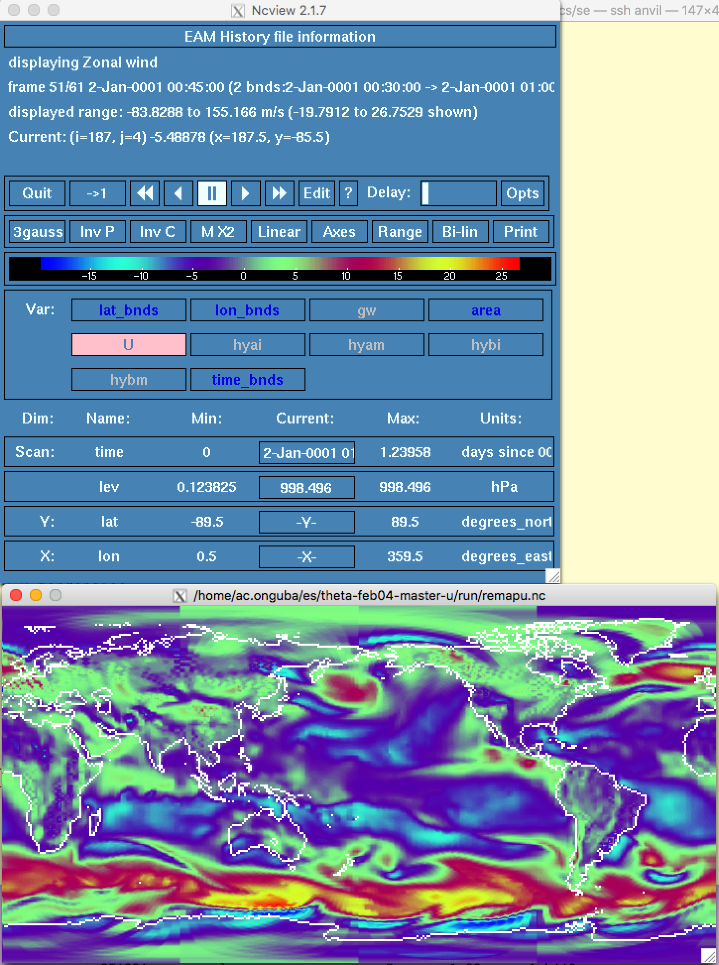
ne30pg2 run, the noise is there, alternating.

[quantheory]

Using a 5 minute time step for the atmosphere also seems OK (green line here).

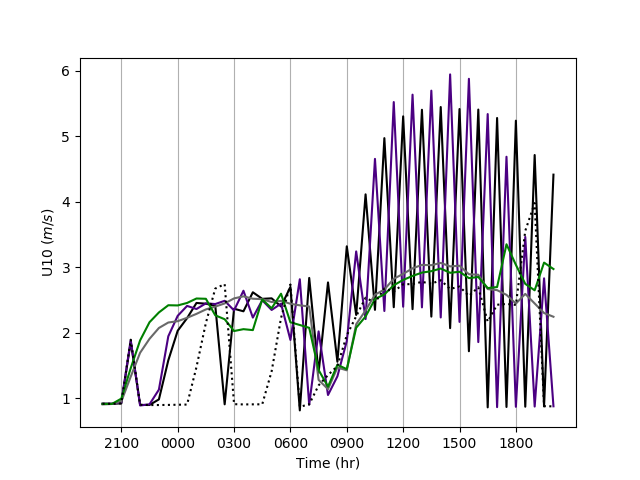
Edit: I made the mistake of not plotting every time step in this plot, so please see below for a better plot of a 5 minute/300 second time step.

[ambrad]

Is there reason to think that leaving dtime=30min but increasing cld_macmic_num_steps to 36 would produce the same result? That might be true if the analysis you apply above models the evolution of u inside CLUBB for fixed a (friction) and b (wind from dynamics).

[oksanaguba]

@ambrad we tried that, see https://acme-climate.atlassian.net/wiki/spaces/COM/pages/1230700892/Third+set+of+runs+it+is+CLUBB -- I tried sub cycling for 100 steps, did not work.

[ambrad]

Thanks. Which part of the code computes the u tendency that oscillates? Can that part of the code be subcycled or, instead, turned into an implicit time step over dtime?

[oksanaguba]

Assuming it is not clubb that produces oscillations, then it is stresses cam_in%wsx, cam_in%wsy , which are computed iirc in coupler and in land(?) (depending on whether it is ocean or land) . Looking at old plots, the noise seems to be only over land.

[ambrad]

I see; thanks. I understand now why this oscillation is an atm-land coupling instability. It makes sense that roughness of land must be substantially larger than the roughness of water. It seems we might want to update the CAM5 implicit surface stress method to work with CLUBB.

[quantheory]

@ambrad I also tried changing cld_macmic_num_steps to 180 (the purple line in the graph), and it does not address the oscillations. As @oksanaguba says, the stresses are computed in the land model, not CLUBB itself. (I assume this is because it depends on information that's only available to the land model, e.g. characteristics of the vegetation.)

I think that the easiest fix for this issue would be to use some kind of flux smoothing over time (either using the sfc_flux_avg option, or something similar, probably adjusted to only apply to the momentum rather than all surface fluxes). This was also a part of the CAM5 implicit surface stress method.

Alternatively, we may be able to fix this by having the land model output enough information to allow the atmosphere to update the stresses (or at least approximate the changes to stresses) in the CLUBB substepping loop. This may lead to consistency issues if the land model and atmosphere model are calculating different surface stresses. On the other hand, conservation of momentum isn't a concern for the land model in the same way as for the atmosphere/ocean models, so maybe it's not that much of a problem.

I also think that we should consider just reducing the land and atmosphere model time steps to a smaller value (somewhere in the 5-15 minute range). But that's mostly because there are other results that might also be improved. This issue alone is probably not enough to justify the extra model cost and retuning that would be needed to reduce the whole atmosphere time step.

[ambrad]

Yes, model efficiency loss is the issue with more frequent coupling.

I like your suggestion of moving the wind stress calculation to the atm. elm/src/biogeophys/CanopyFluxesMod.F90:1176 is an example of how taux,y is computed. There seem to be some parts of the calculation that depend on roughness data R and another part on (u,v), e.g., u*. One could imagine having the land provide a "roughness state" to the atm, having the atm compute subcycled wind fluxes to avoid the oscillations, and then have the atm export wind stress and latent/sensible heat fluxes to the land instead of the opposite. The code itself could of course still live in the land model.

[whannah1]

@ambrad Moving the stress calculation to the atmosphere is not a viable option. Those calculations happen in several different places across the surface components. There's a good chance that there will be additional and/or new surface components in the future too.

I would actually be in favor of reducing the coupling time for ne30pg2 to 15 or 20 min. I can also live with the smoothing option, but I wonder if we can improve it some by smoothing the friction magnitude and adjusting the vector of the residual when it gets applied at the later time step.

[quantheory]

We're unfortunately in a position where we have two relatively "fast" processes, the drag slowing down the lowest layer wind (calculated by the land model), and the propagation of the stresses and other fluxes upwards through the boundary layer (calculated by CLUBB). It would be ideal to integrate these processes together, but that's not straightforward to do given the way the model is set up...

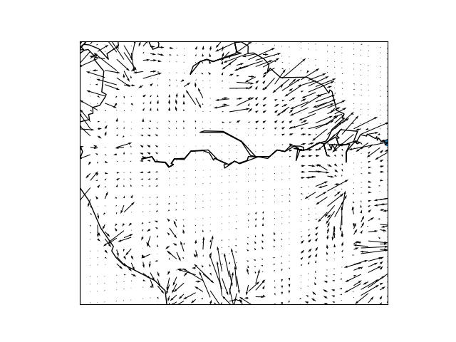
To evaluate the other options, I've done some more runs. First, to show a baseline for what it looks like for the problem to be present, here's a map of the second derivative of the winds with respect to time (via finite differences) in the control run:

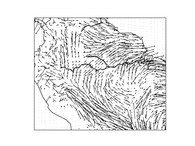
Unless otherwise specified, all of these maps are at about 1200 local time (UTC 0400). Because of the way I've adjusted the scale, basically every grid point with a visible arrow is undergoing large oscillations in the surface winds. This issue is greatly reduced if we reduce the model time step to 300 seconds:

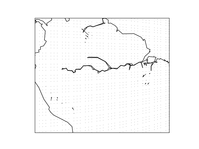
We can also see this by picking an arbitrary grid point and looking at U10 (black is control, grey is a run with 10 second time step, green is a 300 second time step.

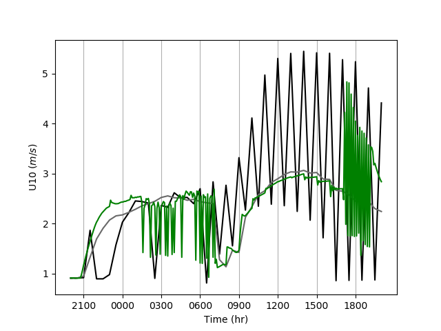
Of course, this does not show that the issue has disappeared, since the oscillations still occur late in the run. Apparently the land roughness can get so large that a 5 minute time step is not good enough to get rid of the oscillations either. But reducing the time step does limit the oscillations to particular times and places. Look at this map of the second derivative of winds at 1800 local time.

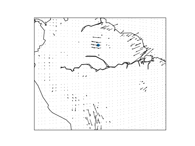
The blue dot marks the point where I am sampling U10 here. While we can see that the second derivative is large while the wind is oscillating, the area of affected land is much smaller than in the control run.

If we use an intermediate time step size of 900 seconds, we still see large second derivatives of wind speed across most of the continent as well:

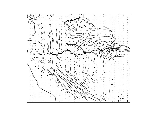
And again you can see this in the time series at one grid point (black dashed line):

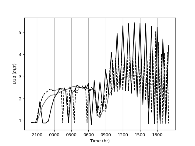
So a 15 minute time step is much worse at addressing this issue than the 5 minute time step.

I've then experimented with various "smoothing"-type modifications. Here was what I got from the sfc_flux_avg option, modified to only apply to surface stresses.

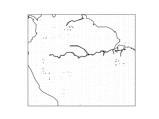
This method is shown as the black dotted line here:

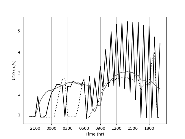
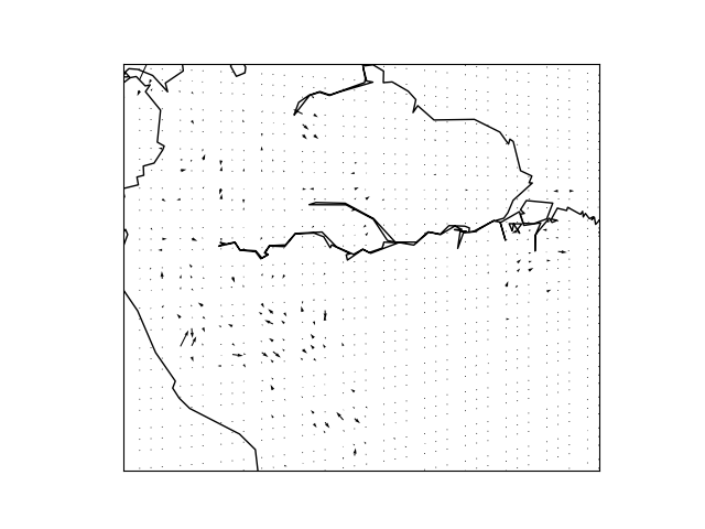
I also tried doing something simpler, which was to apply 3/4 of each stress from the land model at the current time step, and 1/4 in the time step after that. This is more or less equivalent to using an explicit linear multistep method (LMM) with a larger region of absolute stability than the forward Euler method (about twice as large). This shouldn't necessarily work any better than just halving the time step, but it actually does OK:

The LMM variant is shown here in red (the other variant shown in the last plot is also in red, also please ignore the dashed line in this plot):

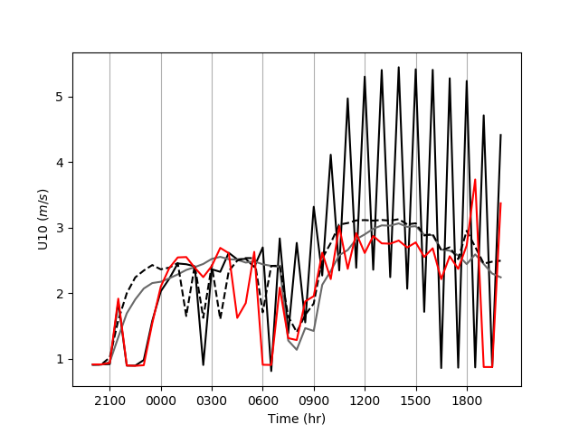
I also tried using an LMM that applies 6/10 of the stress in the current time step, 3/10 in the time step after that, and 1/10 in the time step after that. This does very well:

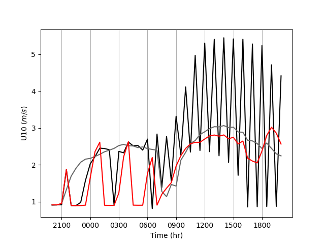
[quantheory]

I know that this was a lot of text/plots, so to summarize:

• A 5 minute time step works much better than a 15 minute time step.
• I found a simple linear method that seems to be as effective at "smoothing" as the older sfc_flux_avg.
• Neither the 5 minute time step nor any of the smoothing methods were completely effective at removing the oscillations. At best, we could make the oscillations much less frequent.

[quantheory]

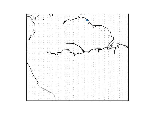
The problem is worse on the coast. Consider this point:

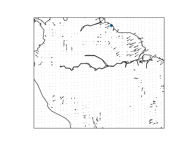
Graphing U10 over two days gives this plot:

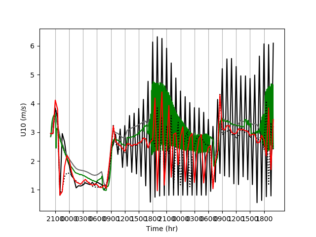
While the original code (black) is the worst, the 5 minute time step (green) has wild oscillations during the night, and the smoothing methods (dotted black = sfc_flux_avg, red = 3 step method) still have some odd oscillations, though it is an improvement (and I notice that the period is >2 time steps in those cases).

[quantheory]

I can mostly fix this problem by both running at a 5 minute time step and using the 3 step method (blue line here).

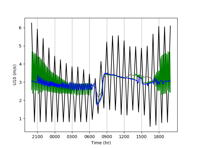
However, we want to solve this without running at a 5 minute time step. If we can't move the surface friction calculations into the same solver as is used to diffuse them through the PBL, I think that we need to consider incorporating more information about the atmospheric dynamics/PBL tendencies into the flux calculations in the land model. The flux calculations need to have some information about how the winds are likely to evolve over the course of the a 30 minute time step, rather than assuming that the instantaneous value of the winds at the beginning of the time step will be maintained for the whole time step.

[whannah1]

@quantheory (just brainstorming here) In the MMF we have an additional problem surrounding friction. For any given column+CRM you get a single friction vector that reflects the GCM wind, but the boundary layer eddies inside the CRM create fluctuations in both directions. It took us awhile to realize that this was causing eddies of a certain vorticity sign to be damped while the opposite sign was amplified, leading to the boundary layer having a tendency to turn into one large overturning circulation within the CRM.

We address this problem by calculating an additional "pseudo friction" using the CRM winds and an estimate of the roughness length. Initially we tried to find a way to make sure that the total friction within the CRM always matches the friction provided by the surface models, but this just led us back to a version of the original problem. The current strategy involves leaving the CRM winds uncoupled from the GCM winds and using a scheme invented by Stefan Tulich where we use special scalars to calculate the CRM momentum transport.

Thinking about this in the context of CLUBB makes me wonder if we could use a similar strategy in which we estimate a roughness length based on the surface momentum fluxes, use that to calculate friction at each CLUBB substep, and then make a correction at the end to make the boundary layer KE dissipation consistent with the total friction vector from the coupler.

There's a lot of hand waving there, but I'm just thinking out loud.

[whannah1]

@quantheory another thought after more MMF tinkering. I have this refactored MMF branch where these friction issues are somewhat amplified. Reducing the time step helps a lot as we would expect. Another thing I tried while I was tinkering was enabling the old "turbulent mountain stress" (TMS) scheme. Jaga Richter pointed me to this paper that talks about it being used in an older version of WACCM, but it appears that it's never been enabled by default in CAM or EAM.
https://journals.ametsoc.org/view/journals/atsc/67/1/2009jas3112.1.xml
Unlike the gravity wave parameterizations that they talk about in that paper, it seems that TMS only adds some extra friction at the surface in mountainous regions. Turning this on made a previously unstable case with dt=20 min look similar to a stable case with dt=10 min. I found some other tweaks and hacks that would get the dt=20 min case running, but none of those tests produced results that were as smooth as the TMS test.

For an example, here's some time step output of U at the bottom model level for a single column from 4 tests:

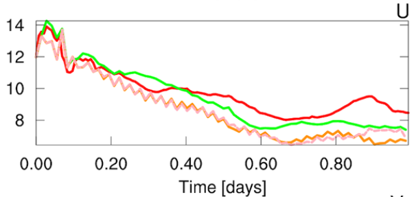
red: dt=10 min
green: dt=20 min + TMS
orange/pink: dt=20 min + (something else I tried to increase boundary layer diffusion)

If I try to run the dt=20 min case in an identical way to the dt=10 min case (with the same underlying 5 min dynamics time step) the run crashes in under 10 time steps, so in all cases changing things in the boundary layer is making a difference.

So I'm tempted to run with TMS enabled... but I'm also very hesitant since it was never used outside of WACCM.

[quantheory]

@whannah1 I think that's interesting, although TMS by itself doesn't help that much for the cases I've been looking at. This is what happens if I just run with default settings and do_tms=.true.:

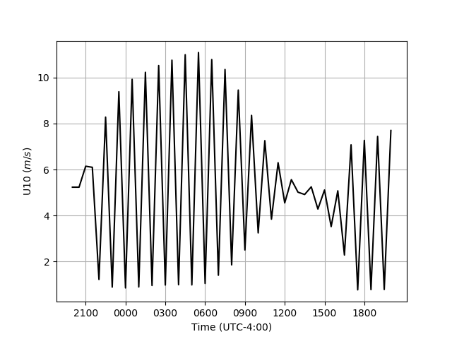
I guess that by adding on the TMS, you're adding on a second source of stress, which is reducing the surface winds enough that the calculations in the land model can settle down a bit. But it doesn't seem to be working in every case.

I think it's worth noting that the oscillations aren't affecting just the lowest level in some cases. In this plot of wind speed, you can see that the fight between the vertical diffusion and the surface stress is strong enough to be whipping the bottom 5-10 levels around every time step.

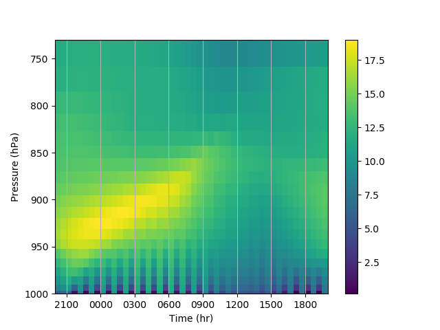
[quantheory]

I have a new E3SM branch with a new set of modifications to deal with this issue, which can be seen in the comparison here:

https://github.com/E3SM-Project/E3SM/compare/master...quantheory/implicit-land-fluxes

These modifications add some extra calculations to CLUBB, which produces some estimated derivatives that allow the land model to predict the effect of fluxes on the state of the lowest level of the atmosphere. This in turn allows the use of implicit methods in the land model to calculate the land-to-atmosphere fluxes.

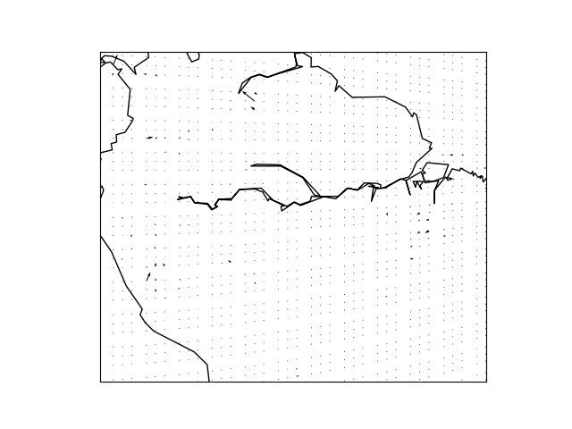
This approach has been somewhat effective so far. Here is the second derivative with respect to time of the winds at a particular moment in a control run:

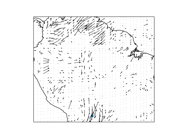
And here is the same snapshot using the implicit land fluxes tag:

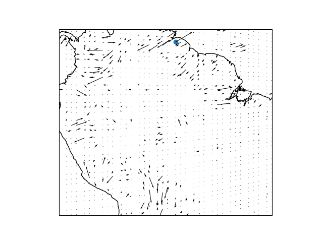
You can also see the effect of these changes in columns that are prone to oscillations. In the following plot, the black line shows an unmodified control simulation, the yellow line uses the implicit flux code for the stresses only, the red line uses the implicit flux code for both stresses and sensible heat and water vapor fluxes, and the grey line uses a second-order (trapezoidal) implicit method for both stresses and fluxes.

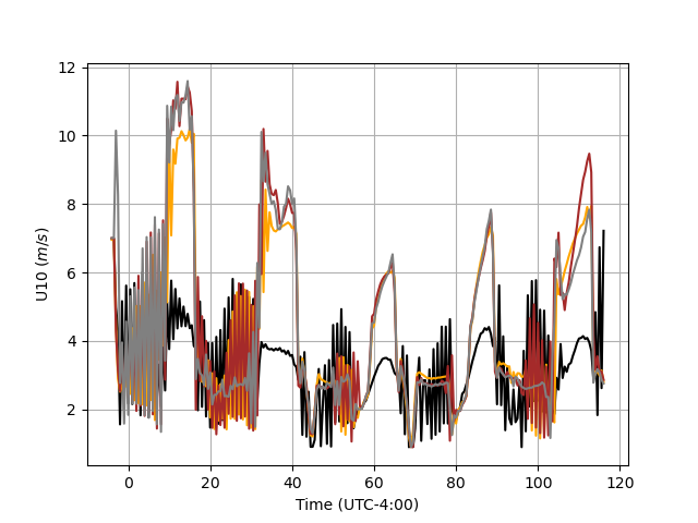
You can see that the implicit flux code is much less prone to oscillations after the first day or two of spinup. However, this particular example is maybe too favorable to the trapezoidal method configuration. In most cases, all three of these implicit flux configurations have similar levels of oscillations, but the trapezoidal method has fluxes that are more similar to the control run in columns that are not prone to oscillations.

The main problems with this code are that it (a) still has some oscillations, and (b) produces stresses that are too small (hence winds that are much too large) in rougher areas. I've done some further poking around at columns that have particularly large oscillations. So far I believe that both of these problems are due to the fact that my modifications to CLUBB do not account for the generation of turbulent kinetic energy from surface stresses (and hence the increase in the model's eddy diffusion). This leads the land model to overestimate the effect that stresses will have when there is relatively little turbulence, and hence produce stresses that are both too small on average, and too variable (because the land is too sensitive to the model's current amount of TKE). I have an idea of how to fix this, which I plan to test in the next week or two.

These code modifications are also quite extensive. I think that many of these changes (in particular the changes to the sensible heat and vapor fluxes) will turn out not to be necessary, though I don't think that there's any problem with them per se.

[quantheory]

@whannah1 Because these modifications depend on outputs I've added to CLUBB, I'm not sure where they fit in with the MMF code. The land mods would probably still work fine for MMF, but you'd need some other way to derive the information needed for the implicit land fluxes.

[whannah1]

@quantheory great stuff! I think this might actually be something we could work into the MMF in some form. The MMF never directly handles the surface stress, it only feels it indirectly via the momentum forcing (if enabled). I recently refactored the MMF to use the older diagnostic PBL scheme from the CAM2/3 day, and we will now have our own version that can freely diverge from E3SM, so I can try to do something similar. I'll wait till you get more experience with this method and then probably ask @lee1046 to think about how we can adapt it to the MMF.

RE: weaker stress over topography - do you think the turbulent mountain stress can be enabled to help this problem?

[quantheory]

I do think that the TMS might help. When I get around to looking at the effect on TKE next week, I might also look at running with the TMS parameterization turned on.

[adamrher]

Hi @quantheory, @tto061 and others have beens discussing your mods for calc. the surface stresses w/in the land model implicitly. We wanted to get your thoughts on Thomas' idea to perhaps linearize about the Ri number (or all prognostic variables that determine the Ri number, T, u, v) the stresses fed to CLUBB, and iterate in CLUBB to allow the MO surface layer to adjust in tandem with the PBL. Some relevant remarks from Thomas:

The reason for my "conceptual doubts", as I called them, is that Sean's approach to finding the correct solution takes more, instead of less, of the problem into the surface components, so in my view it is, in that sense, making the code drift away from the full fix, which would be to to find the correct solution for atmospheric surface flux layer and atmospheric surface turbulent layer in an iteration within the atmosphere.

Conceptually, the surface flux layer self-similarity solution is an equilibrium solution for constant fluxes within a thin layer given a certain prescribed, steady vertical wind shear and thermal stability that are controlled by the PBL. The adjustment time-scale here should be very fast and the available heat and momentum in the flux layer too small to modify the vertical structure it is embedded in, so that the self-similarity assumption is justified. The PBL provides that slowly varying vertical structure by distributing stability and momentum over a thick atmospheric layer.

CAM goes the wrong way about this, by imposing unchanging surface fluxes regardless of the state of the PBL. Bu it is CLUBB that should see an evolving surface-flux layer according to the updated state of the PBL. It should then adjust the PBL state to the changed surface fluxes, with the surface layer calculation never responding to CLUBB tendencies -- lest the self-similarity assumption be broken, invalidating, in principle, the theory that the calculations implement.

I don't think that Sean's solution is therefore wrong in any way. As you say, at core this is a time-stepping issue, so numerical convergence is the key. But to me the corresponding mods seem to fix a broken code by making it even less consistent with what should be the right solution. The surface (=slow) components should never pass fluxes to the atmospheric PBL (=fast); it should always be the other way around.

and

Adam
perhaps the short version of what I'm saying is this:
Instead of iterating in the land models using a linerised CLUBB response to the surface fluxes, iterate in CLUBB, or in micmac, with a approximated reponse of the surface layer. This should be relatively simple, given e.g. tau=-c_D |u|u, where c_D depends only on the Richardson number: so it would be enough to linearise dc_D=dc_D/dRi *dRi.

But the surface flux component would then have to accept that updated flux to advance their state, before calculating the next c_D and its derivative.

What do you think?

[whannah1]

@adamrher It seems this idea might not be applicable in the context to atmos/ocean coupling since the fluxes are calculated in the coupler. It seems that if you passed the coupler an "adjusted" friction that it had to then pass to the ocean, I'm not sure if the ocean could adjust for stresses that were already applied and mixed down in the previous coupling iteration. What do you think?

[adamrher]

@whannah I think that is something that needs to be addressed if we go down this road of adjusting the fluxes in clubb. It sure seems that Sean's method would be easier to achieve the goal of having all component models see the same fluxes by sprinkling the clubb linearization into all component models.

Would @whannah1 and @quantheory be interested in joining a task force-like meeting on implicit fluxes? There are a few of us ncar folks (+Thomas) who are very interested in this topic.

[quantheory]

@adamrher I think that this is timely, since I was thinking of some related issues just yesterday. I do agree with Thomas that an ideal solution would be if CLUBB was able to adjust the surface fluxes. It is not straightforward to implement such a thing though. A lot of the modifications I've been messing around with can be viewed as ways of trying to get the land model to predict how CLUBB would adjust the surface fluxes if it could, to improve stability. I am writing up a few pages that describe my view of the issue, which I think differs from Thomas's a bit (or maybe not; I'm not sure exactly what modifications he is thinking of recently).

I would be interested in a meeting if there are people at NCAR that want to talk about this further. I organized a meeting with a different group a couple weeks ago, but I think that we had... less-than-perfect overlap between the people who were invited/able to attend, and the people who have the strongest interest in working on this directly. (That said, @chaneyn was interested but not able to make it, and I can ask if anyone else in that group wants to be involved other than Walter and Thomas.)

[adamrher]

Hi Sean,

Our different threads are getting hard to follow and Julio wants to make a more organized effort to address this on the ncar side. So I was going to put together a doodle poll to find a common time so that (most) of the following can attend:

Julio Bacmeister
Rich Neale
Thomas Toniazzo
Sean Santos
Walter Hannah
Vince Larson
Meg Fowler
Chris Kruse
Marianna V.

If you can think of others that would like to attend (like @chaneyn) just provide their emails and I'll add them to the doodle poll / mtg announcement.

[oksanaguba]

Would you please add me as well? I'd like to listen. Also, I have 2 questions about surface stress fluxes:

1) my understanding is that they are not energy-conserving. That is, energy conservation is not considered. I was about to add that the corresponding energy leak is probably small, but now I am not sure I measured it properly, outside of clubb.
2) is there a reason to apply the fluxes in clubb? could they be applied independently?

thnaks

[adamrher]

@quantheory I should probably give a little more background. I don't feel like the current implementation of applying the surface fluxes in clubb was all that well thought out, and I and others feel the need to address this dirty laundry. We have seen spurious oscillations similar to what is described in this thread, hence my interests in collaborating on a solution.

I think your approach is so far the best one that has been proposed ... But with the hefty fingerprint in the code mods, I'd like to carefully think out the implications of going down this road in cam. In particular, Julio and I are curious about the implications of (continuing to) break assumptions in self-similarity theory. And Thomas obviously has expressed his concerns as well. And so a brief outline of the proposed meeting would try to understand exactly what challenges exist if we wanted to more tightly couple the surface fluxes with the PBL evolution in CLUBB. It sounds like you've thought about this, and it seems like you're a little more pessimistic on this approach. This is why I wanted to include Marianna in the mtg, to understand what challenges this poses for coupling with the ocean.

But I also want to emphasize that whatever approach we take it needs to be numerically defensible (i.e., stable at long time-steps), and your approach goes a long way towards achieving that goal.

[Edit] One more thing we want to understand is how any changes to the surface flux algorithms impact the CLASP CPT, whose goal is to use the land heterogeneity in CLM to provide surface fluxes of variances and co-variances to clubb.

[adamrher]

@oksanaguba I don't have much to say about 1, but will think about it and probably chat with Peter L about it as well. But for

is there a reason to apply the fluxes in clubb? could they be applied independently?

Yes and no. clubb has an option of the host model providing the surface fluxes to clubb, in which case these fluxes are boundary conditions in the clubb solver. For latent and sensible heat flux, they are solved using a 5-diagonal solver that semi-implicitly solves for the new means and fluxes in the physics column simultaneously. This is what is currently used in CAM.

There is also the option to not provide clubb with the surface fluxes, but I'm not sure how the B.C. are handled in the clubb solver in that case. Presumably this option assumes that the surface fluxes were applied to the atmosphere eleswhere in the code.

[philipwjones]

Haven't been tracking this closely so apologize if these comments miss the mark. But from an ocean/ice view...

The ocean fluxes are a little bit less of an issue. We ocean modelers are used to taking an imposed flux and are often coupling at a slower timescale and averaging the fluxes a little anyway. The main reasons why the surface fluxes are computed in the coupler and not the atmosphere is so that they could be computed on the (typically finer) ocean mesh and so that the coupler could do the time averaging. This all may change if we want to include roughness from a wave model.

The sea-ice is a more serious issue because the sea-ice computes surface fluxes in an integrated implicit solve for the whole temperature profile through the ice. This posed a problem in the past when the UKMO picked up the prior CICE model and had to integrate with their implicit PBL scheme. I think they kludged a surface iteration of some kind. I'm guessing the land model will have more serious objections too.

Oksana brought up the issue of conservation and we do take the conservation of all the fluxes seriously, but much more attention is paid to the heat and water fluxes. We conserve the wind stress during the interpolation, but I don't know that we do a detailed KE budget or look at energy consistency (PE-KE conversion) across the system.

Finally, these fluxes are just the sort of issues we hope to address in the Coupling Approaches for Next Generation Architectures (CANGA) project and we have done some early work on implicit or mixed approaches across these interfaces that don't involve iterating entire components. Unfortunately, all the work has been in very simplified models and we don't have anything to satisfy your immediate needs. Hopefully we'll have some solutions to these kinds of problems in a couple years. You can see some early results from the CANGA overview at the last all-hands.

[quantheory]

Just to give a brief update on this, I've done some pen and paper work, and I think that I have an improved implicit calculation method that (a) is provably stable when run with CLUBB and (b) does not introduce any bias in the surface fluxes compared to the original code. This second point is important, because the first version of the implicit stress code did systematically weaken the surface stresses. I will try and see if I can produce updated code tomorrow.

However, the stability proof only works when the surface stress is calculated just before CLUBB runs. I think this does re-raise the question of whether the coupling should be moved to before CLUBB in the atmosphere loop (or equivalently, if CLUBB and everything after it in tphysbc should be moved to tphysac).

[adamrher]

I think this does re-raise the question of whether the coupling should be moved to before CLUBB in the atmosphere loop (or equivalently, if CLUBB and everything after it in tphysbc should be moved to tphysac).

I've been thinking about this as well. We are discussing plans to experiment with linearization of the surface flux calculations in the model components, and passing those to CLUBB. This requires the surface fluxes computed from a state prior to the CLUBB call, so that winds are balanced, and then we can adjust the stresses in CLUBB, which is seeing a state that is one full time-step ahead of that used to compute the surface fluxes.

The question I've been asking is, the i/o historically see's a state that is after the macrophysics so there is no unrealistic super-saturation in the state. I think it's fine for the CPL to see this imperfect state (?), but not the i/o.

[quantheory]

We are discussing plans to experiment with linearization of the surface flux calculations in the model components, and passing those to CLUBB.

I've just realized that this is also a requirement of the approach I've been working on. I want the CLUBB interface to produce an estimated "equilibrium" stress that the surface would need to generate a roughly steady state. However, in order to do this, I need at least to have the derivative of the surface stress with respect to the magnitude of the lowest-level wind.

[quantheory]

I ended up getting very good results with a much simpler modification to the implicit land fluxes, which was to assume that the boundary layer had reached a solution that was roughly consistent with the surface stress from the previous time step, and thus the difference between the current and previous stress value was the main thing causing the lowest-level wind to change over the next time step.

During the day, this modification basically kills the oscillations entirely, as this map of the second derivative of lowest level wind (at roughly 11 am locally) shows:

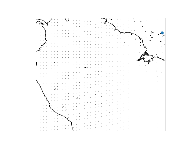
That's the best result I've been able to get without changing the model time step or vertical resolution, and you can see that the least smooth behavior is actually over the ocean (which has not been modified, since I have only implemented the method for the land so far). The picture in the evening (roughly 7 pm) is not as perfect, but still much better than most other things I've tried:

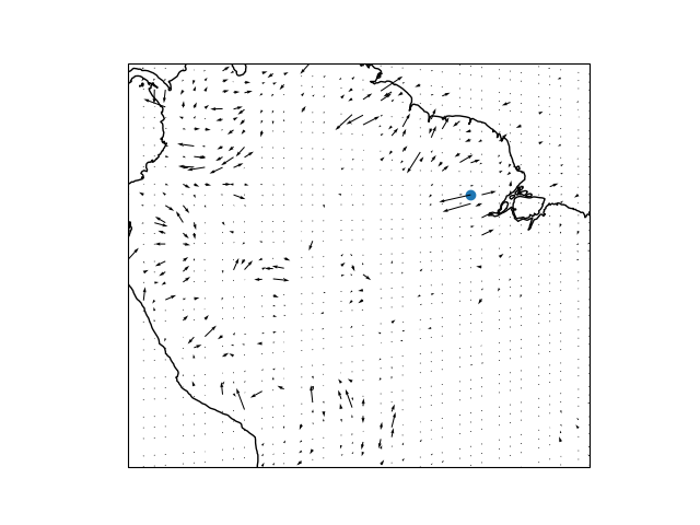
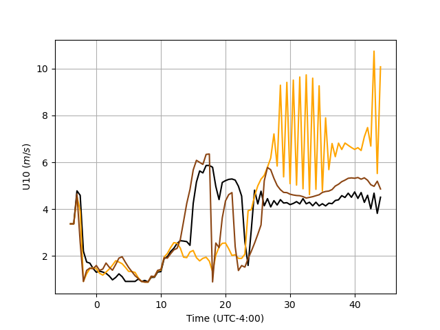
To take some particular case studies, here is U10 for a particular column in the Andes. Black is the control run, yellow is the original implicit flux code, and brown is the new implicit flux code.

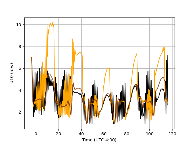
You can see that the new code essentially never produces sustained oscillations. It does produce occasional "spikes", though it's not clear to me whether those are due to the surface stresses themselves, or caused by some kind of external shocks (e.g. from the dynamics). Also, this version tends to produce roughly the same solution as the control run when there are no oscillations (as opposed to the original implicit flux code, which tends to produce much weaker stresses/stronger winds during the day).

Here is another case where the new code does fairly well:

And probably the worst case behavior for the new code:

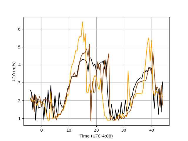
In this last case the new code still doesn't produce sustained "oscillations", but there is a great deal of non-smooth noise. This noise lines up somewhat well with the noise in the surface stress, but the surface stress is sometimes fairly constant for a few time steps when U10 is changing rapidly:

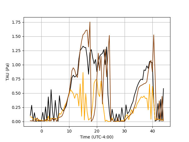
This makes me wonder whether some of the boundary layer oscillations actually come from other atmospheric processes that have trouble with large shear in the boundary layer, rather than being caused by oscillations in the surface fluxes (e.g. something in the dynamics, or the parameterized gravity waves).

I also have started a write-up that explains my view of the situation in more detail, but the current draft has a lot of stuff that's just my "notes" that may not be very clear to anyone else (especially anything past page 10, some of which is probably wrong anyway). Still, if you're curious, you can read that paper here. The main thing I want to point out is that I do have a rough theoretical framework explaining why the oscillations are so severe in the original code, and also showing why the modified code should not have those oscillations at all.

[whannah1]

The question I've been asking is, the i/o historically see's a state that is after the macrophysics so there is no unrealistic super-saturation in the state. I think it's fine for the CPL to see this imperfect state (?), but not the i/o.

Unfortunately, based on my experiments rearranging the atmosphere loop with the MMF, I'm almost positive that it is problematic for the coupler to see a state that has not been adjusted by convection. The presence of super-saturated, or just relatively humid, conditions when coupling just after dynamics leads to a large systematic change in the climate, which affects the latent and sensible fluxes. Ironically, in some areas this seems to help some biases, but overall the MMF moved further from a realistic climate when I did this.

As an alternative, we could consider moving CLUBB to tphysac, or even calling CLUBB twice (both in AC and BC phsyics), but we'll probably just see a different flavor of the same problems.

[adamrher]

@whannah1 That's some useful insight. So then moving CLUBB to tphysac is not an option, as it is the super-saturation adjustment. And if that's the case, then there is no obvious way of getting around the fact that the surface fluxes applied to CLUBB are computed from a state lagged by a time-step ... and the way that Sean and Thomas have been going about fixing this, is the way forward.

An unattractive way to solve this would be to break up the CLUBB scheme so that pdf closure (i.e., the SVP adjustment) is done in tphysbc, but the prognostic equations advanced in tphysac ...

[whannah1]

@quantheory These comparisons with the implicit methods are pretty interesting, but I'm thinking we should also be comparing these results to a case with a shorter coupling interval. I'm guessing the implicit methods will be cheaper, but eventually when we get to some long-term analysis I think it's a natural question to ask whether just shortening the coupling time will get us similar results.

[quantheory]

Hi to everyone watching this thread. I don't see it as a complete solution, but note PR #4229, which is a pull request for the best set of changes I've found so far for this case.