Arviz: autocorr vs autocorrplot

[MFreidank]

This issue is actually more of a question, it is quite possible that we can resolve this without actual code changes. arviz maintains autocorr code in stats.diagnostics._autocorr and plots.autocorrplot (both are inherited from the pymc3 codebase). Both here and in pymc3 the way the autocorrelation is computed differs, in particular plots.autocorrplot uses np.correlate(y, y, mode=2) whereas stats.diagnostics.autocorr uses fftconvolve(y, y[::-1]). Is there a reason why plots.autocorrplot does not simply use stats.diagnostics.autocorr under the hood?

[aloctavodia]

Not sure probably historical reasons, if so It would be wise to follow your suggestion and use stats.diagnostics.autocorr. Maybe @junpenglao can provide further insight.

[ahartikainen]

I think they have updated the correlate function in numpy. I think we should use the one which is faster.

n = 100, 1000, 10000, 100000, 1e6

[ColCarroll]

Ooh, maybe the opposite of historical reasons. I believe I was porting this to use xarray, and wanted to avoid plt.acorr, which used to be used: it does not add much to the code complexity, but allows a lot more flexibility in signature and styling. I did not even notice az.diagnostics._autocorr!

Checking out benchmarks and actual values, it looks like the two functions are not identical, but are quite close where there is actual autocorrelation, and that az.diagnostics._autocorr is much faster for large inputs, and modestly slower for small ones. I attached the code below. Trying np.correlate on 1e6 points scares my computer.

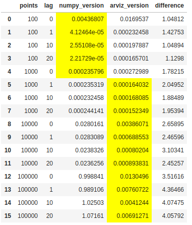
def numpy_version(y):
    points = len(y)
    z = np.correlate(y, y, mode=2)[points - 1:]
    return z / z[0]

metrics = []
for j in range(2, 6):
    points = 10 ** j
    y = np.random.randn(points)
    for lag in (0, 1, 10, 20):
        metrics.append({'points': points, 'lag': lag})
        z = y.copy()
        if lag:
            z[:-lag] = z[:-lag] + z[lag:]
        t0 = time.time()
        a = numpy_version(z)
        metrics[-1]['numpy_version'] = time.time() - t0
        t0 = time.time()
        b = az.diagnostics._autocorr(z)
        metrics[-1]['arviz_version'] = time.time() - t0
        metrics[-1]['difference'] = np.linalg.norm(a - b)

[ahartikainen]

fft version will automatically calculate for all lags which is great.

[MFreidank]

@ColCarroll I might have wanted to be more complete in my initial question.. blame it on the haste I had while writing it ;)
I do think that the argument of "historical reasons" is somewhat applicable regardless: plt.acorr uses np.correlate(y, y, mode=2) under the hood, so your refactoring did not change that part of the behavior, it only improved the interface.

I already had a prior suspicion that this might be efficiency-related given that effective_n requires plenty of autocorrelation-related computation.
I guess phrasing my original question a bit clearer:
Does anything speak against using az.diagnostics._autocorr in az.plots.autocorrplot?

It seems to scale better, it is readily available and it makes the interface more consistent overall.
If you want I can start working on a pull request to change np.correlate(y, y, mode=2) to az.diagnostics._autocorr inside az.plots.autocorrplot. I would definitely include some comparisons old version vs new version so that we can ensure the difference in actual plots is negligible.

[ColCarroll]

Yes, changing to use az.diagnostics._autocorr (and perhaps changing the name of that to remove the leading underscore!) would be great.

I had not realized how expensive the calculation would be in numpy, to crash my computer with 1e6 points (which we _probably_ won't have from MCMC, but should also probably support that case).

I'm more concerned about the difference in the actual calculations now, though. Maybe my numpy_version above is incorrect, but here's an example:

x = np.random.randn(5).cumsum()
print(numpy_version(x))
print(az.diagnostics._autocorr(x))

[1.         0.60192985    0.3577708     0.41361888 0.3014416 ]
[ 1.          0.23051673 -0.90943384 -0.5289727    0.36418002]

[MFreidank]

@ColCarroll Oh yes, I must have missed that at first glance. This indeed seems problematic. If your numpy_version is incorrect, then so is matplotlib.acorr, because I have extracted their implementation in matplotlib.axes._axes.Axes.acorr into the following function:

def matplotlib_xcorr(x, y, normed=True, detrend=mlab.detrend_none,
              usevlines=True, maxlags=10, **kwargs):
        if "hold" in kwargs:
            warnings.warn("the 'hold' kwarg is deprecated", mplDeprecation)

        Nx = len(x)
        if Nx != len(y):
            raise ValueError('x and y must be equal length')

        x = detrend(np.asarray(x))
        y = detrend(np.asarray(y))

        c = np.correlate(x, y, mode=2)

        if normed:
            c /= np.sqrt(np.dot(x, x) * np.dot(y, y))

        if maxlags is None:
            maxlags = Nx - 1

        if maxlags >= Nx or maxlags < 1:
            raise ValueError('maxlags must be None or strictly '
                             'positive < %d' % Nx)

        lags = np.arange(-maxlags, maxlags + 1)
        c = c[Nx - 1 - maxlags:Nx + maxlags]
        return c

def matplotlib_version(x):
    symmetric_corr = matplotlib_xcorr(x, x, maxlags=None)
    return symmetric_corr[len(symmetric_corr) // 2:]    # MFreidank: minor change to avoid returning symmetric correlations

I get:

x = np.random.randn(5).cumsum()
print(az.diagnostics._autocorr(x))
print(numpy_version(x))
print(matplotlib_version(x))

array([ 1.        ,  0.38954274, -0.17005044, -0.92680692, -1.69440579])
array([ 1.        ,  0.42546903,  0.14994005, -0.03725146, -0.04436978])
array([ 1.        ,  0.42546903,  0.14994005, -0.03725146, -0.04436978]))

So your numpy_version and matplotlib.acorr agree exactly, whereas az.diagnostics._autocorr produces different values. Is there a bug in the implementation? If so , this might be worth escalating up the chain to pymc3 too as this definitely would also impact effective_n diagnostics.

Update
Further research led me into the stan::math c++ codebase, which seems to share origin with
az.diagnostics._autocorr as it gives the exact same results as this function.

In summary we have:
numpy_version(x) == matplotlib_version(x) != (az.diagnostics._autocorr(x) == stan::math::autocorrelation(x))

Update2
Using acf in R I can match results from matplotlib and numpy_version, but not from az.diagnostics._autocorr:

acf(x, demean=FALSE, plot=FALSE)   # this reproduces `matplotlib` behaviour exactly.

For a moment I was tempted to believe that this is an issue of demean=TRUE vs demean=FALSE but it does not appear to be that, as I can not reproduce az.diagnostics._autocorr with either parameter.

Which raises the question: where does the difference between matplotlib/R and pymc3/stan come from and which version shall we follow?

[MFreidank]

I have found where the differences between numpy_version and az.diagnostics._autocorr come from.
The following version of az.diagnostics._autocorr gives exactly the same results as numpy_version, matplotlib.acorr and R::acf:

def _autocorr(x):
    """
    Compute autocorrelation using FFT for every lag for the input array
    https://en.wikipedia.org/wiki/autocorrelation#Efficient_computation

    Parameters
    ----------
    x : Numpy array
        An array containing MCMC samples

    Returns
    -------
    acorr: Numpy array same size as the input array
    """
    # y = x - x.mean()  MFreidank: removed to reproduce `matplotlib.acorr`
    y = np.asarray(x)
    # len_y = len(y)  MFreidank: removed to reproduce `matplotlib.acorr`
    result = fftconvolve(y, y[::-1])
    acorr = result[len(result) // 2:]
    # acorr /= np.arange(len_y, 0, -1)  MFreidank: removed to reproduce `matplotlib.acorr`
    acorr /= acorr[0]
    return acorr

So now my question appears to be: Why are the lines I commented in my code above there?
The first one seems obvious: it detrends the series by its mean, but I'm not sure I understand the intention behind:

acorr /= np.arange(len_y, 0, -1)

[ahartikainen]

I think there are multiple schools for this. (See numpy docstring).

That last arange step is needed in my opinion (it simulates the overlap between the two signals). Also x-x.mean() is just doing mean centering and doesn't affect the fft (0th item only).

What's the difference with n>100?

Please also see what Stan is doing. There was also some discussion about the autocorrelation in Stan discourse (few months ago)

[MFreidank]

@ahartikainen
I saw that docstring, though the difference here seems to be of different nature (at first sight to me anyways..). Could you elaborate on "it simulates the overlap between the two signals"? I'm not sure I fully understand that part yet. I fully agree as far as mean centering goes.
Stan definitely does what az.stats.diagnostics._autocorr does. Both have had recent changes in this area in February though, so I should probably carefully study the conversation thread for that.
I will report differences for n > 100 tomorrow. Currently the only real difference between implementations is the np.arange step -- otherwise they are the same up to mean centering (which the previous code in az.plots.autocorrplot was also doing!). If we are sure the np.arange step is correct, I think it is a good idea to remove any inconsistency and use az.stats.diagnostics._autocorr in az.autocorrplot directly. I have code for this ready so if everyone agrees this is a good idea I would be glad to provide a PR.

[junpenglao]

Is the autocorr code from pymc3? If so I wrote it this way so the result is closest to the result in stan https://github.com/pymc-devs/pymc3/pull/2854

[EDIT] as @ahartikainen said, there are different ways to compute autocorrelation (the simplest being the cross correlation using np.corr), but the current implementation should be the most appropriate for computing the auto-correlation and autocov of MCMC chain.

[junpenglao]

On the implementation side, you can see this notebook: https://nbviewer.jupyter.org/gist/junpenglao/aa6ea70d55d1c93fc11e45e3bf8666bd/Check%20Effective%20Sample%20Size.ipynb

On the theory side, you can follow the discussion in https://github.com/stan-dev/stan/issues/2450

[MFreidank]

@junpenglao yes it is from pymc3. I noticed that it gives the same results as pystan. Thanks for providing background on the implementation and theory. I think it makes sense to use this method to compute autocorrelation in az.plots.autocorrplot as well. I will provide a pull request for that tomorrow.

[MFreidank]

Fixed in #143.